Lecture 10

Julia Schedler

Announcements

Assignment 1 due next Monday night at Midnight
Posted some time today or tomorrow morning
Midterm grades by next Monday
A note on AI use
Grading update

Recall the “Time series data analysis process”

Observation
Question
Hypothesis
Experiment
Data Collection and Analysis
Conclusion
Report Results
Replication

“Observations” of the day

Activity 1: Define a question

Research Questions of the Day

What is the estimated value of the Quarterly Adjusted GNP for 2002, Q4?
What is the estimated percent of Egyptian GDP due to exports in 2018?

Note: These are both forecasting questions.

Methodological Questions of the Day

When do we want to fit an ARMA model?
When do we want to fit an ARIMA model?
How do we identify the order(s) of the ARIMA(p,d,q) model?
How can we check assumptions of a model?
How do we compare models?
How can we forecast from a model?

Definition of ARMA model

A time series \(x_t\) is ARMA(p,q) if

\[ x_t = \alpha + \phi_1 x_{t-1} + \phi_2 x_{t-2} + \dots + \phi_p x_{t-p} + w_t + \theta_1 w_{t-1} + \theta_2 w_{t-2} + \dots + \theta_q w_{t-q} \] Where \(\phi_p \ne 0, \theta_q \ne 0, \sigma^2_w > 0\) (and the model is causal and invertible)

Causal and invertible? 😱

For “causal”, if the time series is stationary it has a causal representation (depends on past, not future)
For “Intertible”, it’s so the moving average part gives us a unique model

A note non-uniqueness of Moving Average

Consider the MA model and its theoretical autocorrelation function, where \(\sigma^2_w\) is the white noise variance

\[ \begin{aligned} x_t &= w_t + \theta w_{t-1}\\ \gamma(h) &= \begin{cases} (1+\theta^2)\sigma^2_w & \Vert h \Vert = 0 \\ \theta \sigma^2_w & \Vert h \Vert = 1 \\ 0 & \Vert h \Vert > 1 \end{cases} \end{aligned} \] Consider two possible values for \(\theta\) and \(\sigma^2_w\):

\(\theta = 5, \sigma^2_w = 1\)

\[ \gamma(h) = \begin{cases} (1+5^2)\cdot1 & \Vert h \Vert = 0 \\ 5\cdot 1 & \Vert h \Vert = 1 \\ 0 & \Vert h \Vert > 1 \end{cases} \]

\(\theta = 1/5, \sigma^2_w = 25\)

\[ \gamma(h) = \begin{cases} (1+(1/5)^2)\cdot 25 & \Vert h \Vert = 0 \\ 1/5\cdot 25 & \Vert h \Vert = 1 \\ 0 & \Vert h \Vert > 1 \end{cases} \]

Both simplify to \[ \gamma(h) = \begin{cases} 26 & \Vert h \Vert = 0 \\ 5 & \Vert h \Vert = 1 \\ 0 & \Vert h \Vert > 1 \end{cases} \]

In practice we cannot distinguish the difference between the two models (they are stochastically the same). So, we will choose the invertible model, which is the one with \(\sigma^2_w =25\), \(\theta = 1/5\) (see Shumway and Stoffer page 72-73, example 4.6 for details.)

Interpretation of ARMA model

If we let \(\epsilon_t = w_t + \theta_1 w_{t-1} + \theta_2 w_{t-2} + \dots + \theta_q w_{t-q}\), then if \(x_t\) is ARMA(p,q), \[ x_t = \alpha + \phi_1 x_{t-1} + \phi_2 x_{t-2} + \dots + \phi_p x_{t-p} + \epsilon_t \]

Recognize the linear regression structure?
Difference: constraints on \(\phi, \theta\).

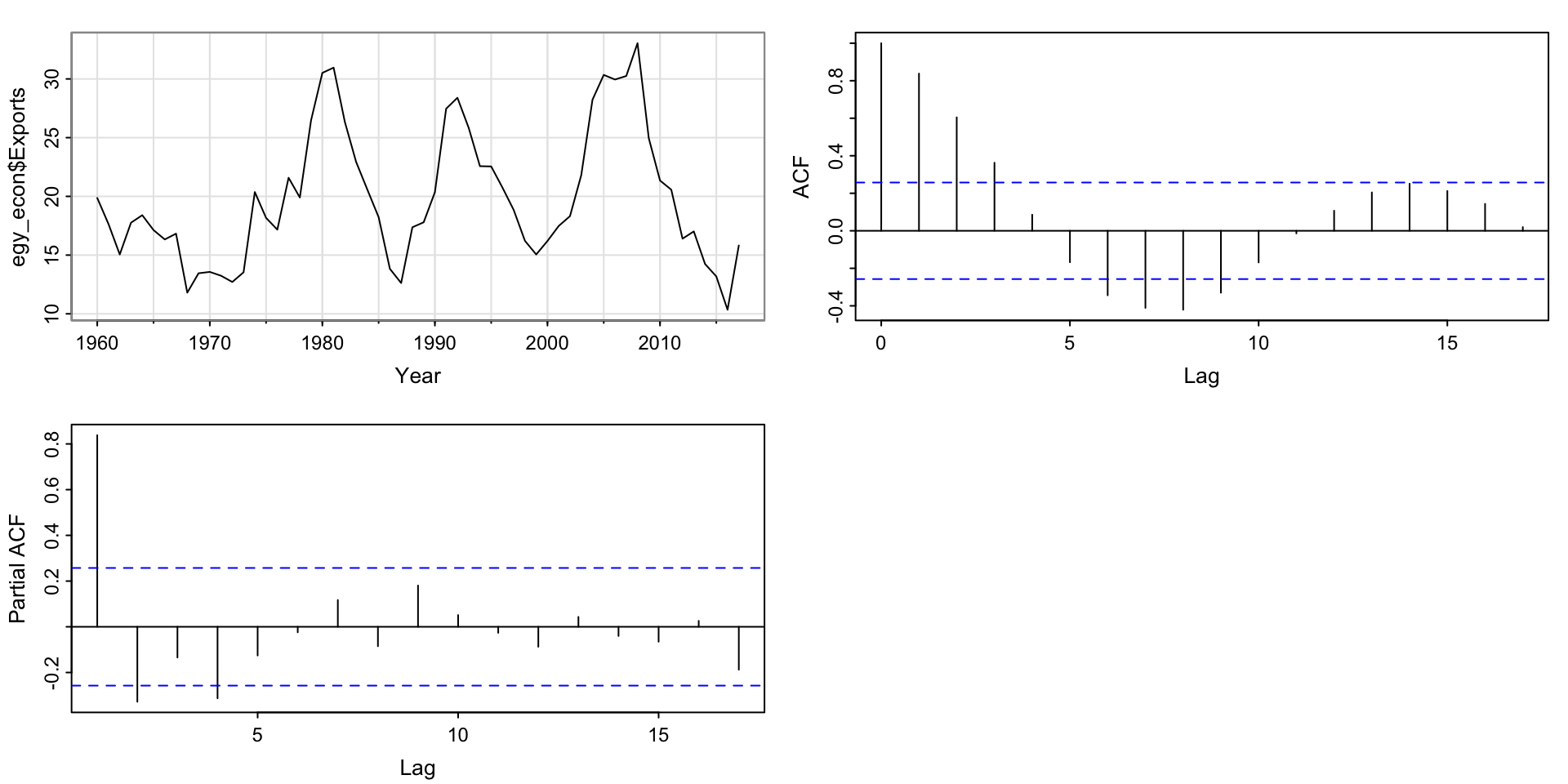
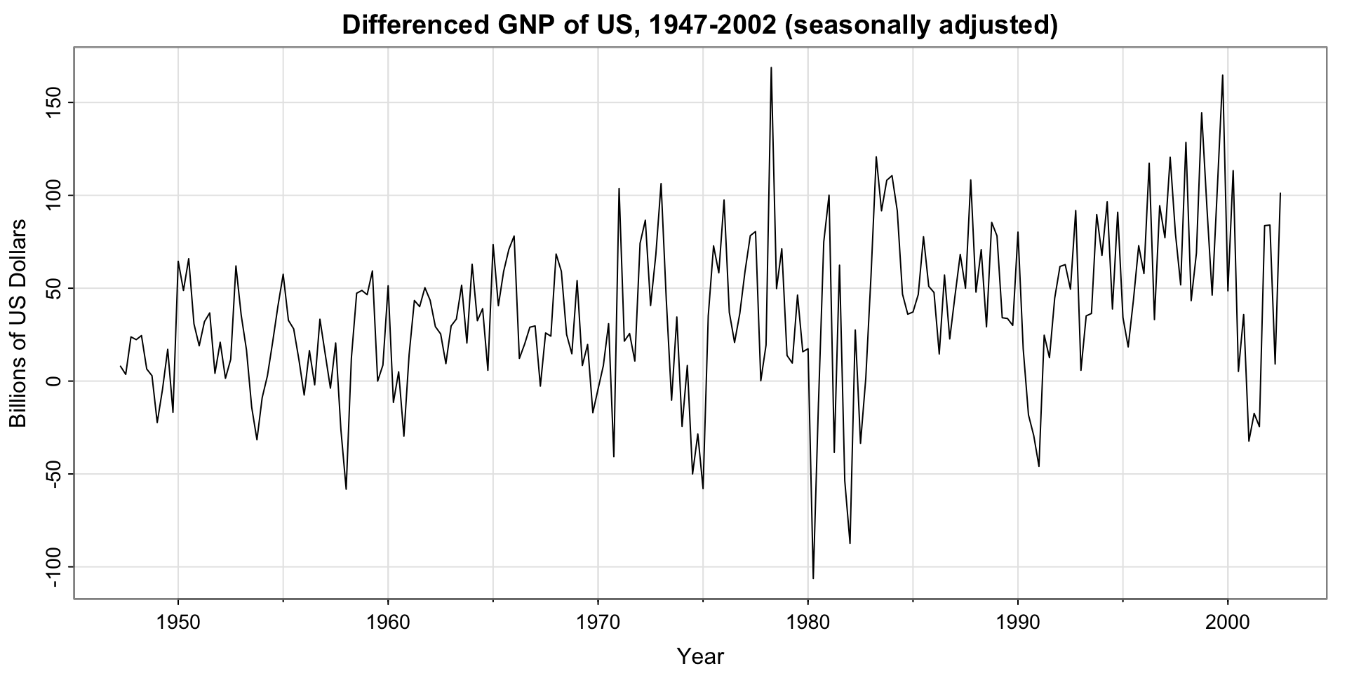
Activity 2: Fit an ARMA model?

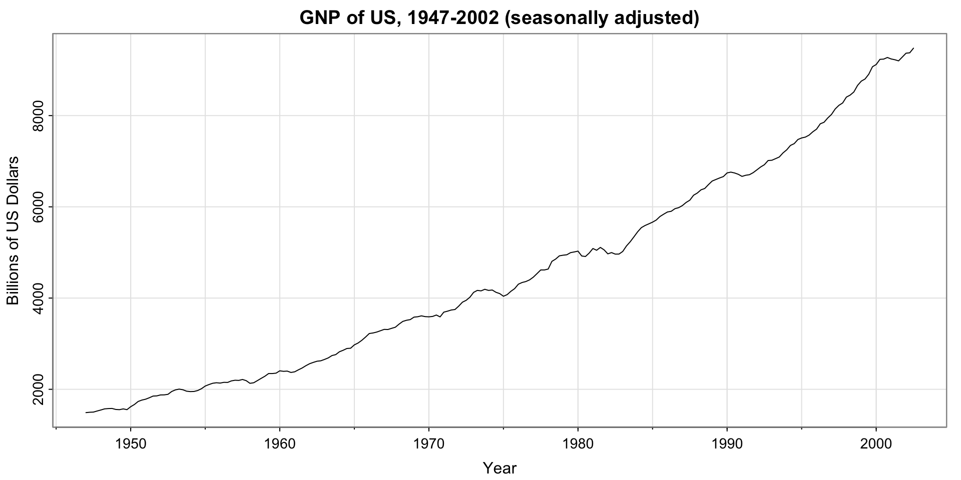
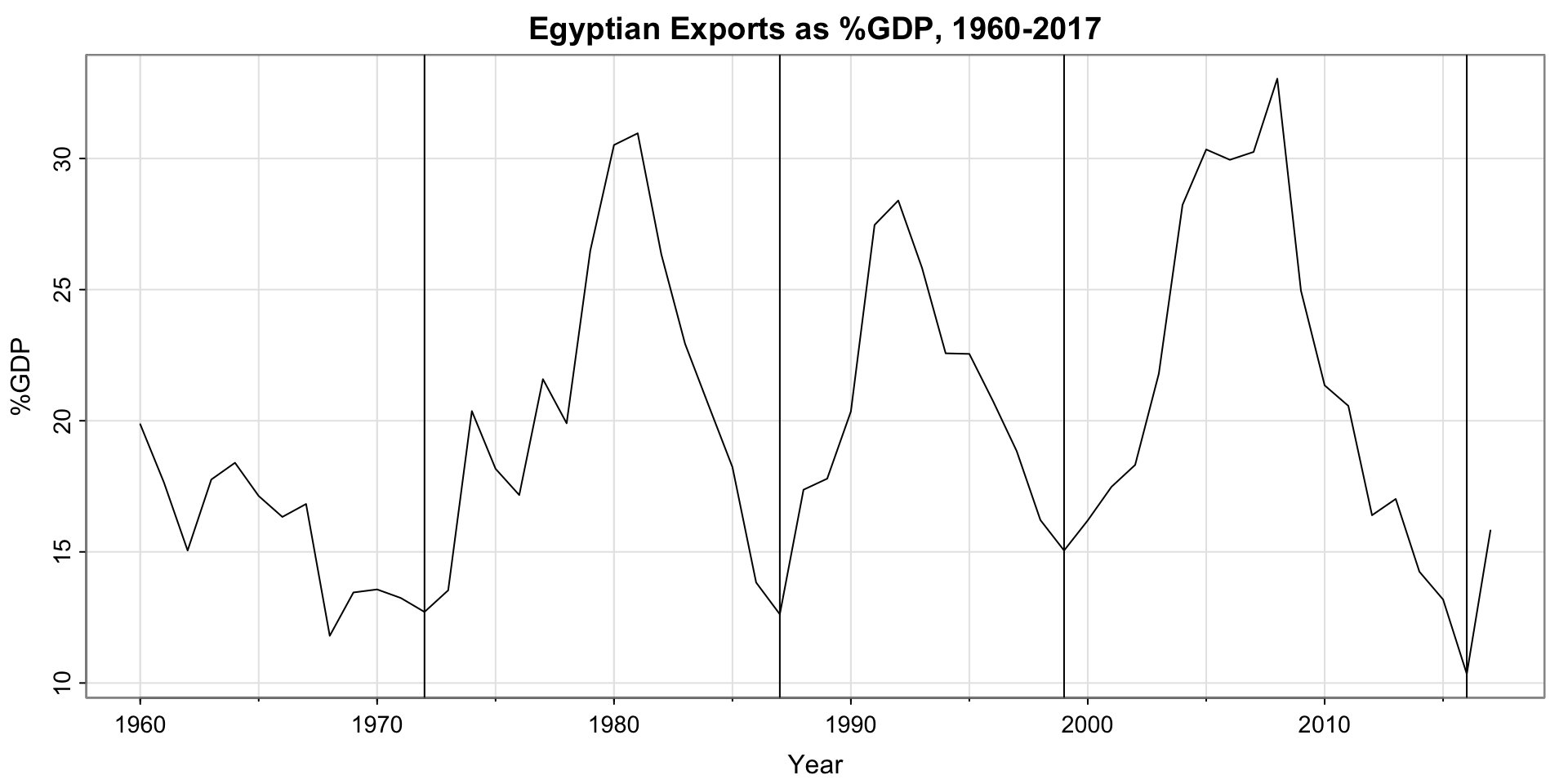
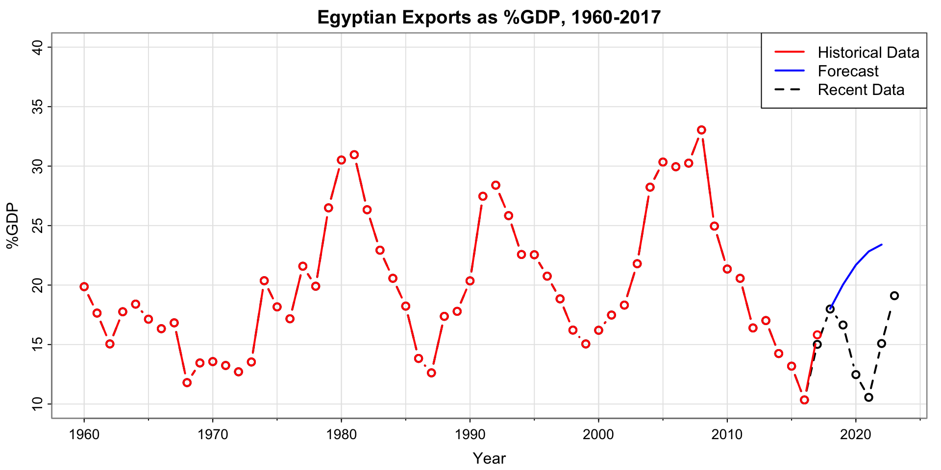
Is there any seasonality (fixed-length cycles)? If so, probably want to use a seasonal model (not ARMA)

Activity 2 Solution: Fit an ARMA model?

No, the cycles are not of fixed length

[1] 15 12 17

Choosing the order of ARMA models

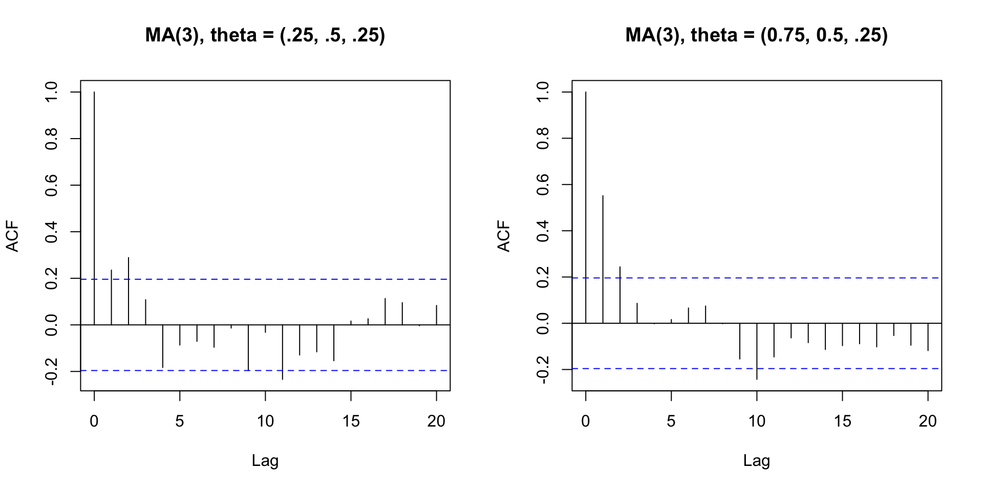
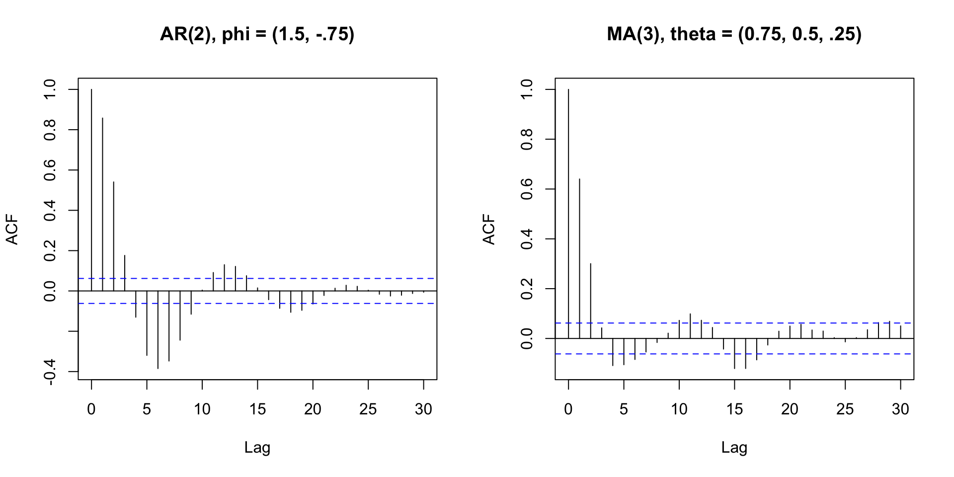
Activity 3: Recall MA ACF

Propose a rule for choosing the order of the MA model.

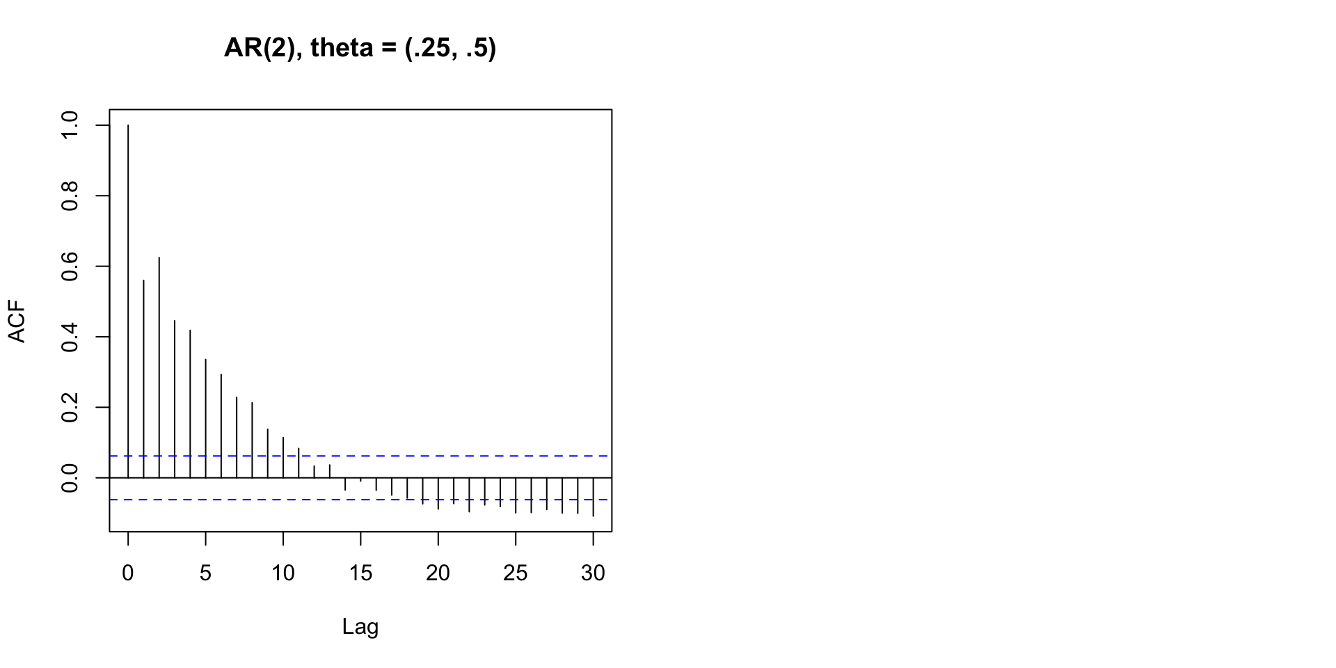
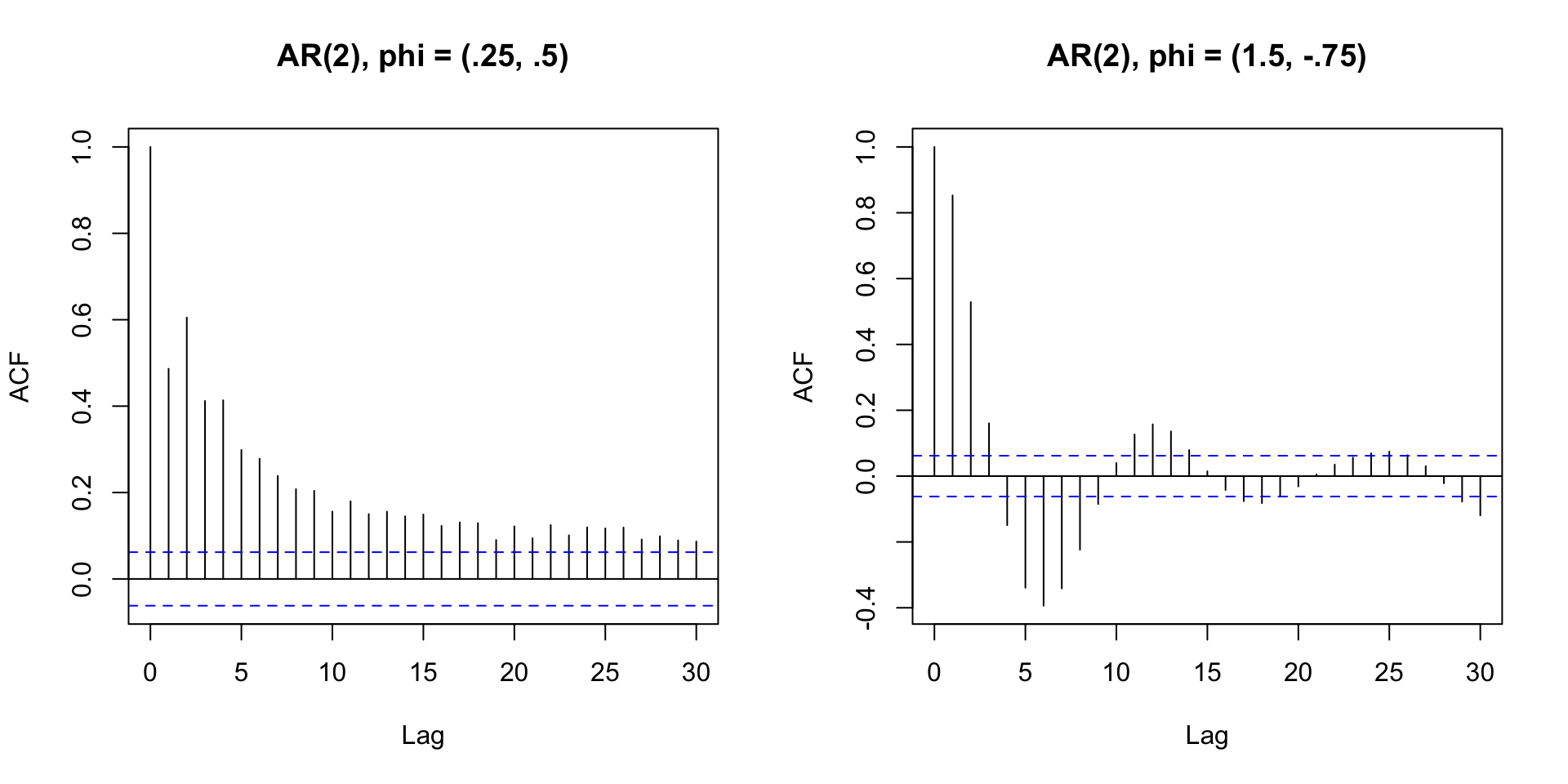
What about AR?

Error in arima.sim(list(ar = c(0.75, 0.5)), n = 1000): 'ar' part of model is not stationary

Activity 4: Fix the AR model so it is stationary

Code

set.seed(807)
par(mfrow = c(1,2))
acf(arima.sim(list(ar = c(0.25, 0.5)), n = 1000), main = "AR(2), theta = (.25, .5)")
acf(arima.sim(list(ar = c(FIXME, FIXME)), n = 1000),
    main ="AR(2), theta = (FIX, FIX)") #hint (lecture 1)

Activity 4 Solution: Fix the AR model so it is stationary

Making sure AR is stationary

Is complicated
Is taken care of in estimation by software

AR or MA or both?

Consider two of the models just simulated:

Shape is similar, but not identical
Is there a better way to tell?

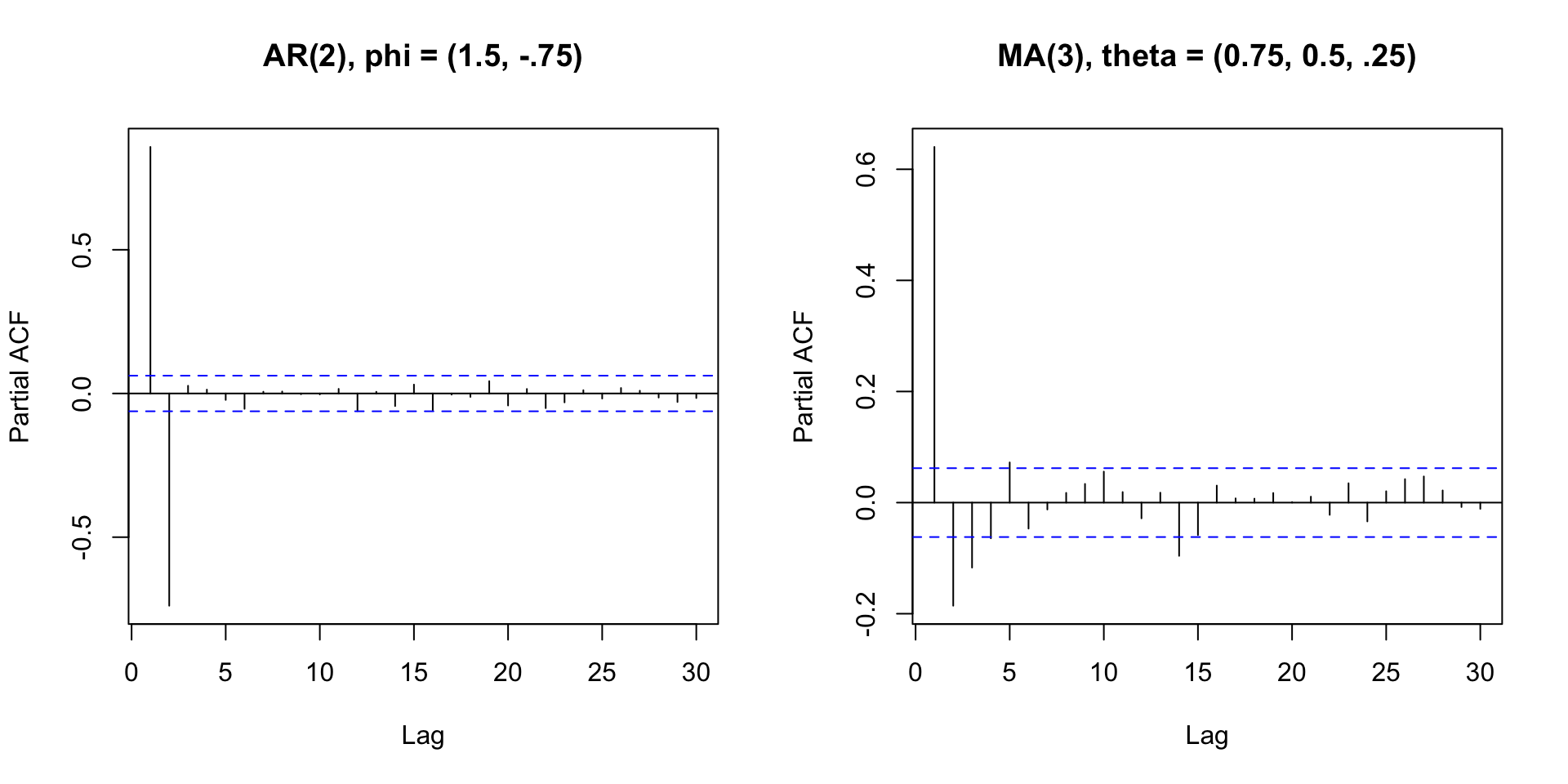
Partial Autocorrelation plot

The PACF is the correlation between \(x_t\) and \(x_{t-k}\) that is not explained by lags \(1, 2, \ldots, k-1\).

“Removes” the autocorrelation of the previous lags.

Useful in determining the order of an Autoregressive process, and in combination with ACF, choosing between an AR or an MA model.

PACF of two series we just saw

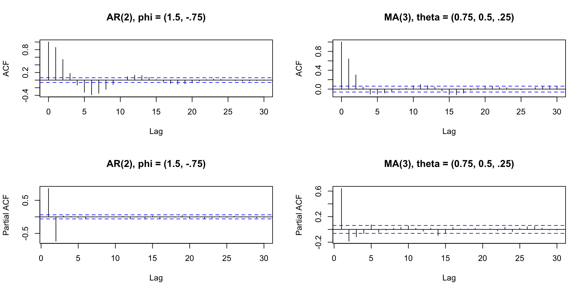
ACF and PACF

AR or MA or both

Behavior of ACF/PACF for ARMA Models
	AR(p)	MA(q)	ARMA(p,q)
ACF	Tails off	Cuts off after lag q	Tails off
PACF	Cuts off after lag p	Tails off	Tails off

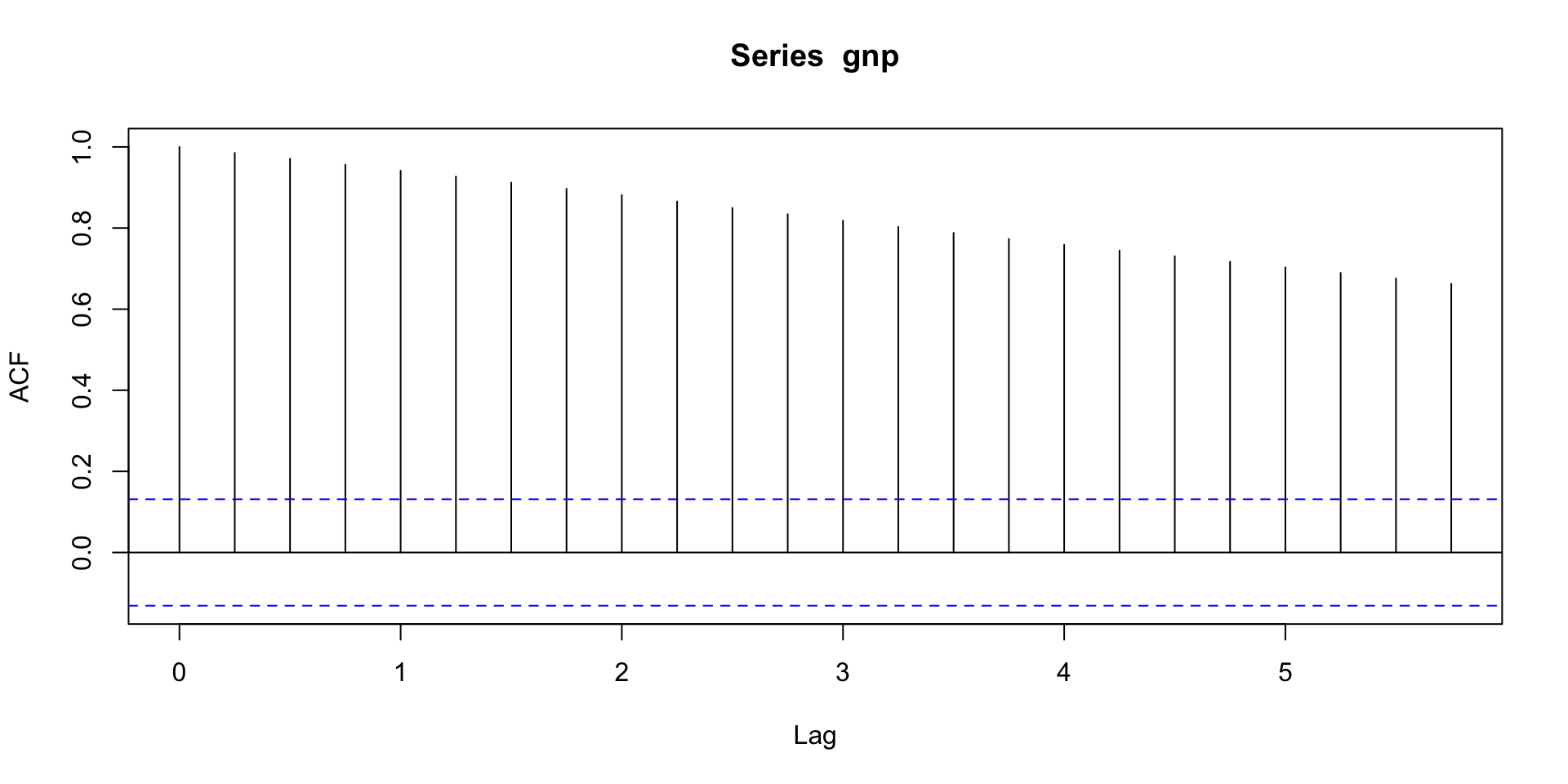
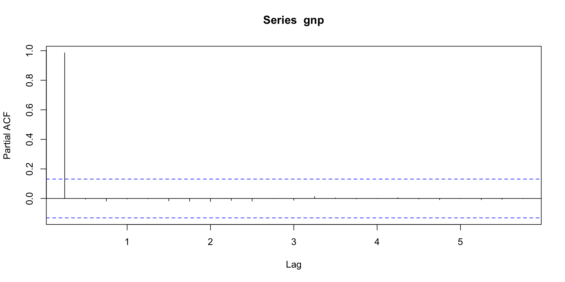
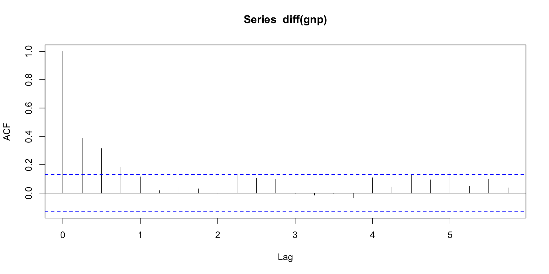
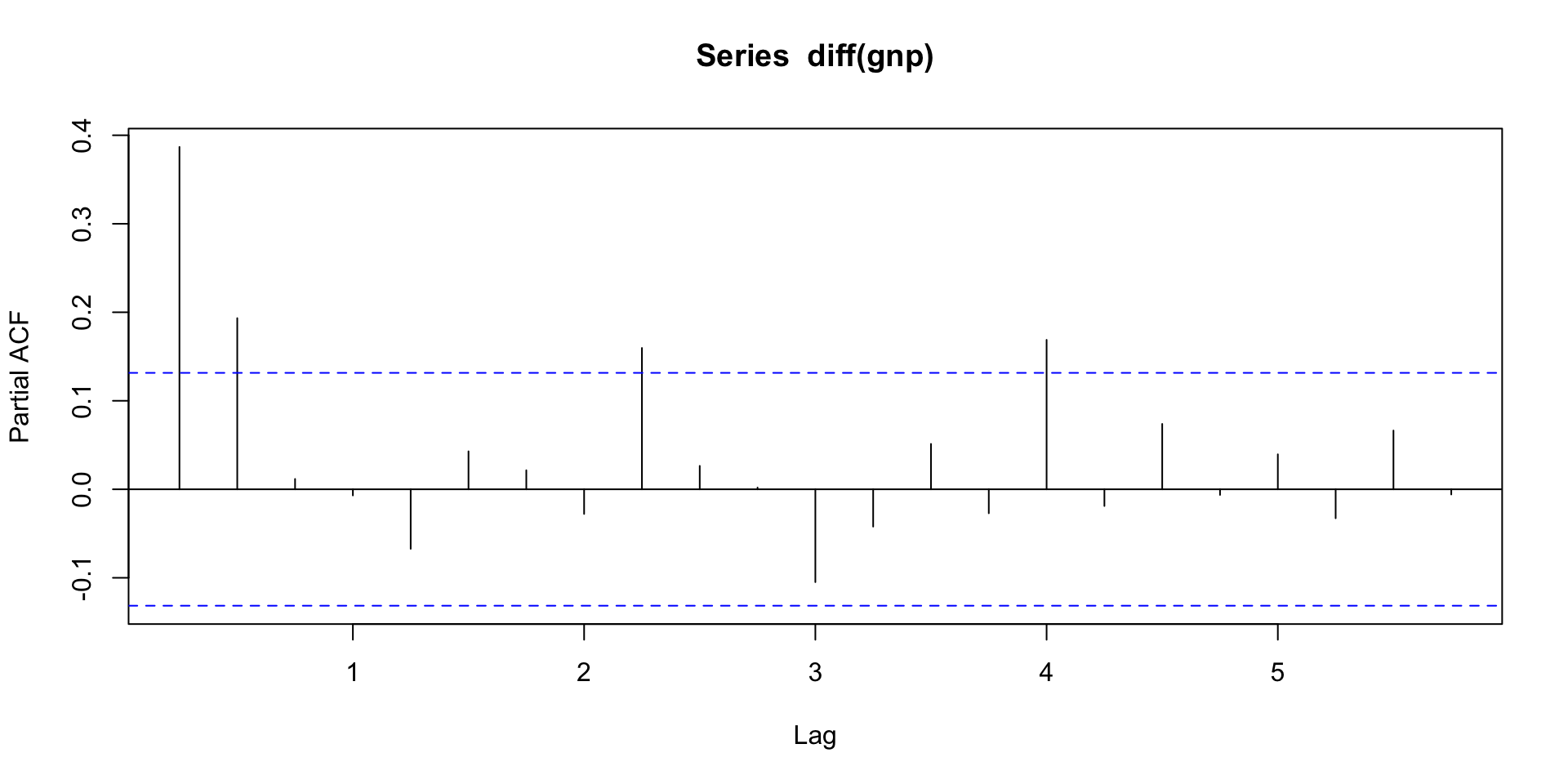
Activity 5: AR or MA or both?

ACF: Tails off; PACF: Cuts off after lag 4. Maybe an AR(4), or some sort of ARMA?

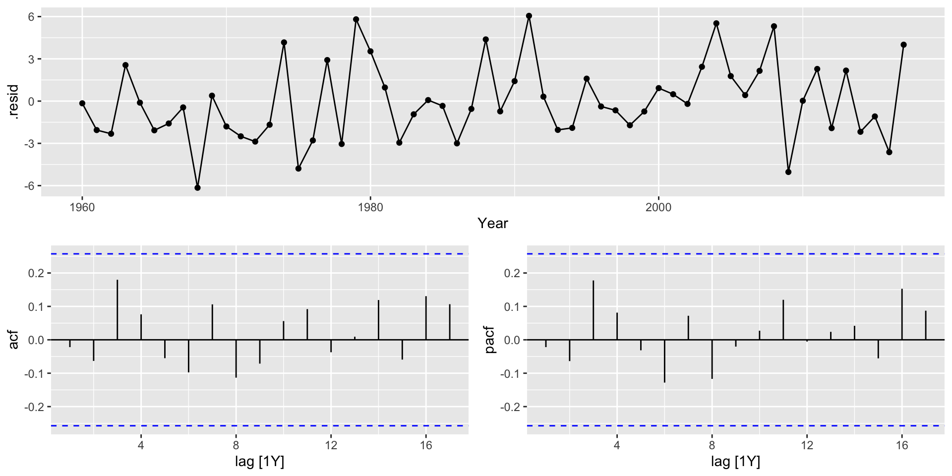
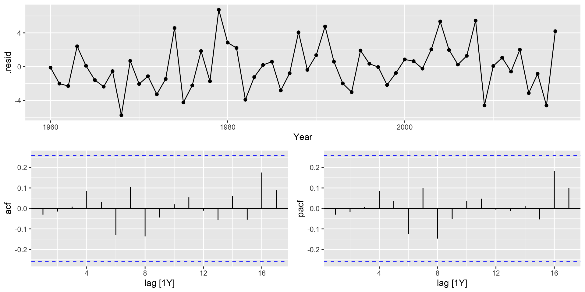
Fitting an ARMA model

Use the sarima function, specify p, d, q (d = 0 for ARMA).

<><><><><><><><><><><><><><>
 
Coefficients: 
      Estimate     SE t.value p.value
ar1     0.9861 0.1247  7.9103  0.0000
ar2    -0.1715 0.1865 -0.9199  0.3618
ar3     0.1807 0.1865  0.9688  0.3370
ar4    -0.3283 0.1273 -2.5779  0.0128
xmean  20.0986 1.0699 18.7858  0.0000

sigma^2 estimated as 7.204995 on 53 degrees of freedom 
 
AIC = 5.052611  AICc = 5.072505  BIC = 5.265761

FPP way

Code

fit_auto <- global_economy |>
  filter(Code == "EGY") |>
  model(ARIMA(Exports)) ## automatic ARIMA
report(fit_auto)

Series: Exports 
Model: ARIMA(2,0,1) w/ mean 

Coefficients:
         ar1      ar2      ma1  constant
      1.6764  -0.8034  -0.6896    2.5623
s.e.  0.1111   0.0928   0.1492    0.1161

sigma^2 estimated as 8.046:  log likelihood=-141.57
AIC=293.13   AICc=294.29   BIC=303.43

Which model should we choose?

One that fits well
We can use AICc to choose between models that seem to have good fit

AR(4) vs. ARMA(2,1)

Series: Exports 
Model: ARIMA(2,0,1) w/ mean 

Coefficients:
         ar1      ar2      ma1  constant
      1.6764  -0.8034  -0.6896    2.5623
s.e.  0.1111   0.0928   0.1492    0.1161

sigma^2 estimated as 8.046:  log likelihood=-141.57
AIC=293.13   AICc=294.29   BIC=303.43

Series: Exports 
Model: ARIMA(4,0,0) w/ mean 

Coefficients:
         ar1      ar2     ar3      ar4  constant
      0.9861  -0.1715  0.1807  -0.3283    6.6922
s.e.  0.1247   0.1865  0.1865   0.1273    0.3562

sigma^2 estimated as 7.885:  log likelihood=-140.53
AIC=293.05   AICc=294.7   BIC=305.41

Very similar! Let’s check the residuals

Check model fit

Code

gg_tsdisplay(residuals(fit_auto), plot_type = "partial")

Code

gg_tsdisplay(residuals(fit_manual), plot_type = "partial")

Make a forecast

Code

fit_auto %>% 
   forecast(h=5) |>
  autoplot(global_economy)

Code

fit_manual %>% 
   forecast(h=5) |>
  autoplot(global_economy)

Code

egy_forecast <- ## save auto forecast 
fit_auto %>% 
   forecast(h=5)

How did the forecasts do?

Plot analysis

the historic data and the updated data mostly agree, except for the last shared point in 2017
The forecast for 2018 is spot-on
The later forecasts are not at all correct

Modeling workflow

GNP Series Example

GNP series

Does the series appear stationary?

Acf and pacf of GNP

Differenced GNP series

Does the series appear stationary?

ACF and PACF of differenced GNP series

ARIMA models

A time series is said to be ARIMA(p,d,q) if

\[ \nabla^dx_t = (1-B)^dx_t \]

Is ARMA(p,q). In other words, if after an order \(d\) difference we get an ARMA model. To bring in the parameters, we write

\[ \phi(B)(1-B)^dx_t = \alpha + \theta(B)w_t \]

Here, \(\phi(B) = 1 - \phi_1B - \phi_2B^2 - \dots - \phi_p B^p\) and \(\theta(B) = 1 + \theta_1 B + \theta_2 B^2 + \dots + \theta_q B^q\)

Example: ARIMA(1,1,0):

Since \(q = 0\), \(\theta(B) = 1\). Since \(q = 1\), \(\phi(B) = 1-\phi_1B\). Finally, \(d = 1\) so

\[ \begin{aligned} \phi(B) (1-B)^dx_t &= \alpha + \theta(B) w_t \\ (1 - \phi_1B)(1-B)^1x_t &= \alpha + 1\cdot w_t\\ (1- \phi_1B)(x_t -x_{t-1}) &= \alpha + w_t \\ x_t - x_{t-1} - (\phi_1Bx_t + \phi_1Bx_{t-1}) &= \alpha + w_t \\ x_t - x_{t-1} - (\phi_1x_{t-1} + \phi_1x_{t-2}) &= \alpha + w_t \\ x_t - x_{t-1} &= \alpha + \phi_1(x_{t-1} - x_{t-2}) + w_t \end{aligned} \]

Next time

More on ARMA vs. ARIMA
Box-cox transformations
Parameter redundancy
Portmanteau tests
Unit root tests
(maybe) Seasonal ARIMA?