Check the page totals (bottom corner) and exam totals (first page)
Find where you lost the most points. What did you do incorrectly?
What was something you did well?
Fill out the canvas Quiz
R code for SARIMA models
sarima function from the astsa package
auto.arima function from the forecast package
model function from the fable package
Which to use??? They all are fine, but output the model object differently, so the model output won’t work with functions from other packages.
Example: Trying to use sarima output with fable diagnostics
You get an error!
Code
library(fpp3)library(astsa)log_gnp <-log(gnp)sarima_model <-sarima(log_gnp, p =1, d =1, q =0, P =0, D =0, Q =0, details =FALSE)## <><><><><><><><><><><><><><>## ## Coefficients: ## Estimate SE t.value p.value## ar1 0.3467 0.0627 5.5255 0## constant 0.0083 0.0010 8.5398 0## ## sigma^2 estimated as 9.029576e-05 on 220 degrees of freedom ## ## AIC = -6.446939 AICc = -6.446692 BIC = -6.400957 ## diagnostics <- sarima_model |>residuals() |>ACF() |>gg_tsdisplay()## Error in UseMethod("measured_vars"): no applicable method for 'measured_vars' applied to an object of class "NULL"
Example: trying to use fable output with sarima diagnostics
Since sarima outputs diagnostics when you fit the model, you could just re-fit the model with sarima and then use the diagnostics.
Code
fable_model <- log_gnp |>as_tsibble() |>model(ARIMA(value ~pdq(1,1,0) +PDQ(0,0,0))) |>report()## Series: value ## Model: ARIMA(1,1,0) w/ drift ## ## Coefficients:## ar1 constant## 0.3467 0.0054## s.e. 0.0627 0.0006## ## sigma^2 estimated as 9.136e-05: log likelihood=718.61## AIC=-1431.22 AICc=-1431.11 BIC=-1421.01sarima(fable_model) ## doesn't work## Error in sarima(fable_model): argument "d" is missing, with no default
Code
## fit the same model, but with default details = TRUE.sarima(log_gnp, p =1, d =1, q =0, P =0, D =0, Q =0)
initial  value -4.589567
iter   2 value -4.654150
iter   3 value -4.654150
iter   4 value -4.654151
iter   4 value -4.654151
iter   4 value -4.654151
final  value -4.654151
converged
initial  value -4.655919
iter   2 value -4.655921
iter   3 value -4.655921
iter   4 value -4.655922
iter   5 value -4.655922
iter   5 value -4.655922
iter   5 value -4.655922
final  value -4.655922
converged
<><><><><><><><><><><><><><>

Coefficients:
         Estimate     SE t.value p.value
ar1        0.3467 0.0627  5.5255       0
constant   0.0083 0.0010  8.5398       0

sigma^2 estimated as 9.029576e-05 on 220 degrees of freedom

AIC = -6.446939  AICc = -6.446692  BIC = -6.400957
Activity 2: Putting it all together
Download “ARIMA code cheat sheet.docx” from Canvas
Pick one column
Fill in the blanks with the correct functions
Forecasting
Given the data and a model that fits the data, we want to predict future values
How can we do this - by “hand” (or just “manually” using code) - using fable or astsa functions
Also, how do we plot these forecasts?
Forecasting using fable or astsa functions
fable functions
Fit model using model() and ARIMA()
Forecast using forecast() specifying h
Code
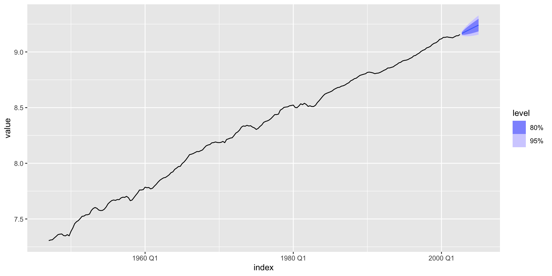
fit <- log_gnp |>as_tsibble() |>model(ARIMA(value ~pdq(1,1,0) +PDQ(0,0,0))) ## force nonseasonalfit |>forecast(h =10)
Determine model order using acf/pacf, check model fit using sarima
Use sarima.for to forecast (with order you chose– re-fits model)
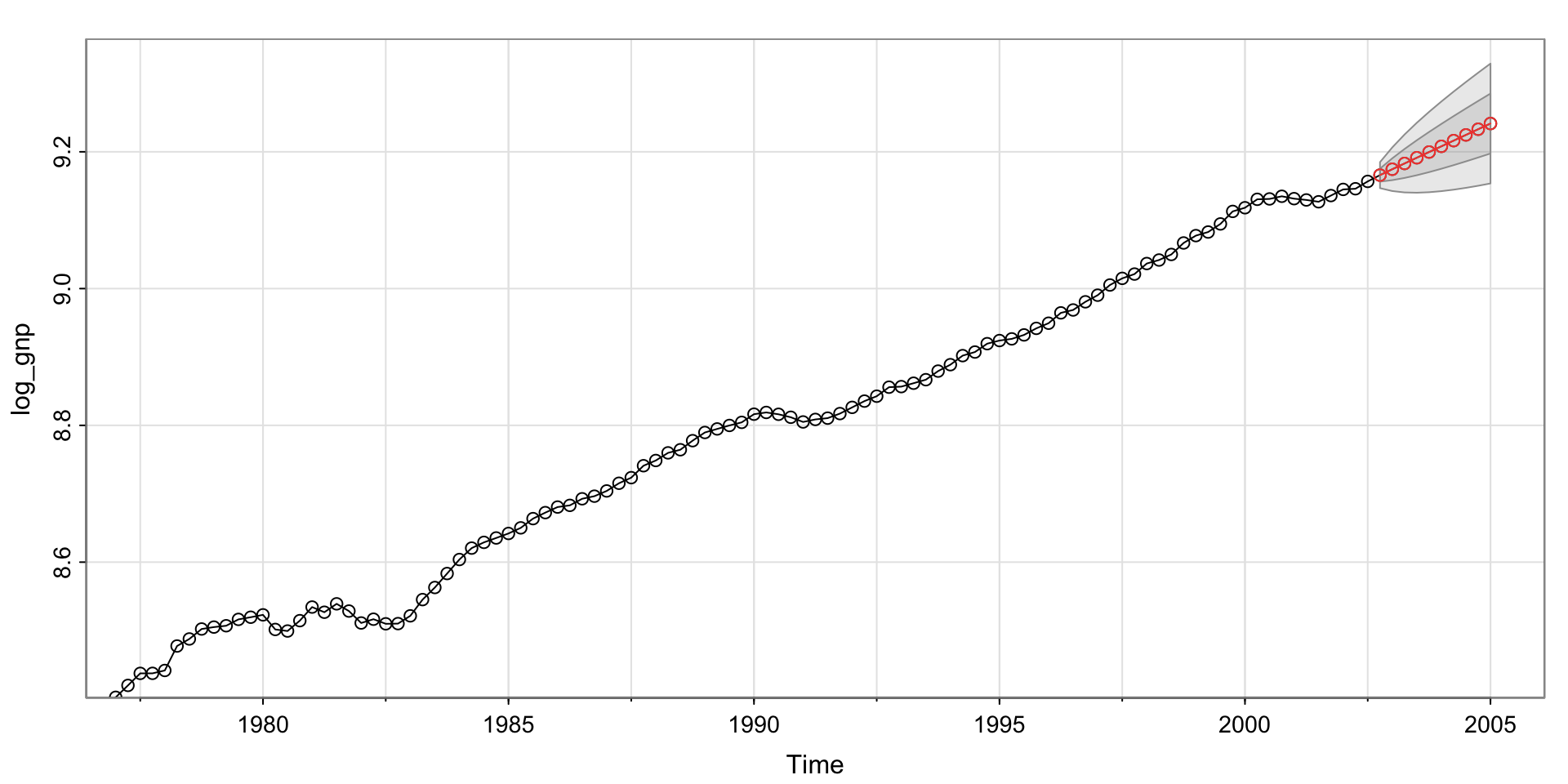
Code
sarima_model <-sarima(log_gnp, p =1, d =1, q =0, P =0, D =0, Q =0)
initial  value -4.589567
iter   2 value -4.654150
iter   3 value -4.654150
iter   4 value -4.654151
iter   4 value -4.654151
iter   4 value -4.654151
final  value -4.654151
converged
initial  value -4.655919
iter   2 value -4.655921
iter   3 value -4.655921
iter   4 value -4.655922
iter   5 value -4.655922
iter   5 value -4.655922
iter   5 value -4.655922
final  value -4.655922
converged
<><><><><><><><><><><><><><>

Coefficients:
         Estimate     SE t.value p.value
ar1        0.3467 0.0627  5.5255       0
constant   0.0083 0.0010  8.5398       0

sigma^2 estimated as 9.029576e-05 on 220 degrees of freedom

AIC = -6.446939  AICc = -6.446692  BIC = -6.400957
Code
sarima.for(log_gnp,p =1, d =1, q =0, P =0, D =0, Q =0, n.ahead =10, plot = F)
\[
(1 - \phi B)(1-B)y_t = c + error
\] Ignoring the error since we want a forecast of the mean, applying the backwards shift operator, F.O.I.L., using our estimate of \(\phi\), and solving for \(y_t\) we get:
\[
\hat{x}_t = x_{t-1} + \hat{\phi}(x_{t-1} - x_{t-2}))+ c
\]
## for fable9.156718+0.3467*(9.156718-9.145983) +0.0054
[1] 9.16584
Code
## for sarima9.156718+0.3467*(9.156718-9.145983) +0.0083
[1] 9.16874
That’s better, but only fable matches the forecast functions?
Comparing constants
Takeaway: Different packages estimate the “constant” differently!
See https://otexts.com/fpp3/arima-r.html#understanding-constants-in-r.
Code
library(fpp3)library(astsa)log_gnp <-log(gnp)fable_model <- log_gnp |>as_tsibble() |>model(ARIMA(value ~pdq(1,1,0) +PDQ(0,0,0))) ## force nonseasonalfable_model |>report()## Series: value ## Model: ARIMA(1,1,0) w/ drift ## ## Coefficients:## ar1 constant## 0.3467 0.0054## s.e. 0.0627 0.0006## ## sigma^2 estimated as 9.136e-05: log likelihood=718.61## AIC=-1431.22 AICc=-1431.11 BIC=-1421.01sarima_model <-sarima(log_gnp, p =1, d =1, q =0, P =0, D =0, Q =0, details = F)## <><><><><><><><><><><><><><>## ## Coefficients: ## Estimate SE t.value p.value## ar1 0.3467 0.0627 5.5255 0## constant 0.0083 0.0010 8.5398 0## ## sigma^2 estimated as 9.029576e-05 on 220 degrees of freedom ## ## AIC = -6.446939 AICc = -6.446692 BIC = -6.400957 ## mu =mean(diff(log_gnp))mu*(1-sarima_model$fit$coef[1])## ar1 ## 0.005447277
Actual by-hand forecast equations:
For fable, where \(c\) is the constant outputted. \[
\hat{x}_{2002 Q4} = x_{2002 Q3} + \hat{\phi}(x_{2002 Q3} - x_{2002 Q2}))+ c_{fable}
\]
For astsa, where \(c\) is the constant outputted. \[
\hat{x}_{2002 Q4} = x_{2002 Q3} + \phi(x_{2002 Q3} - x_{2002 Q2}))+ mean(diff(x_t))(1 - \hat{\phi})
\]
Code
## for astsa9.156718+0.3467*(9.156718-9.145983) +mean(diff(log_gnp))*(1-0.3467)
[1] 9.165887
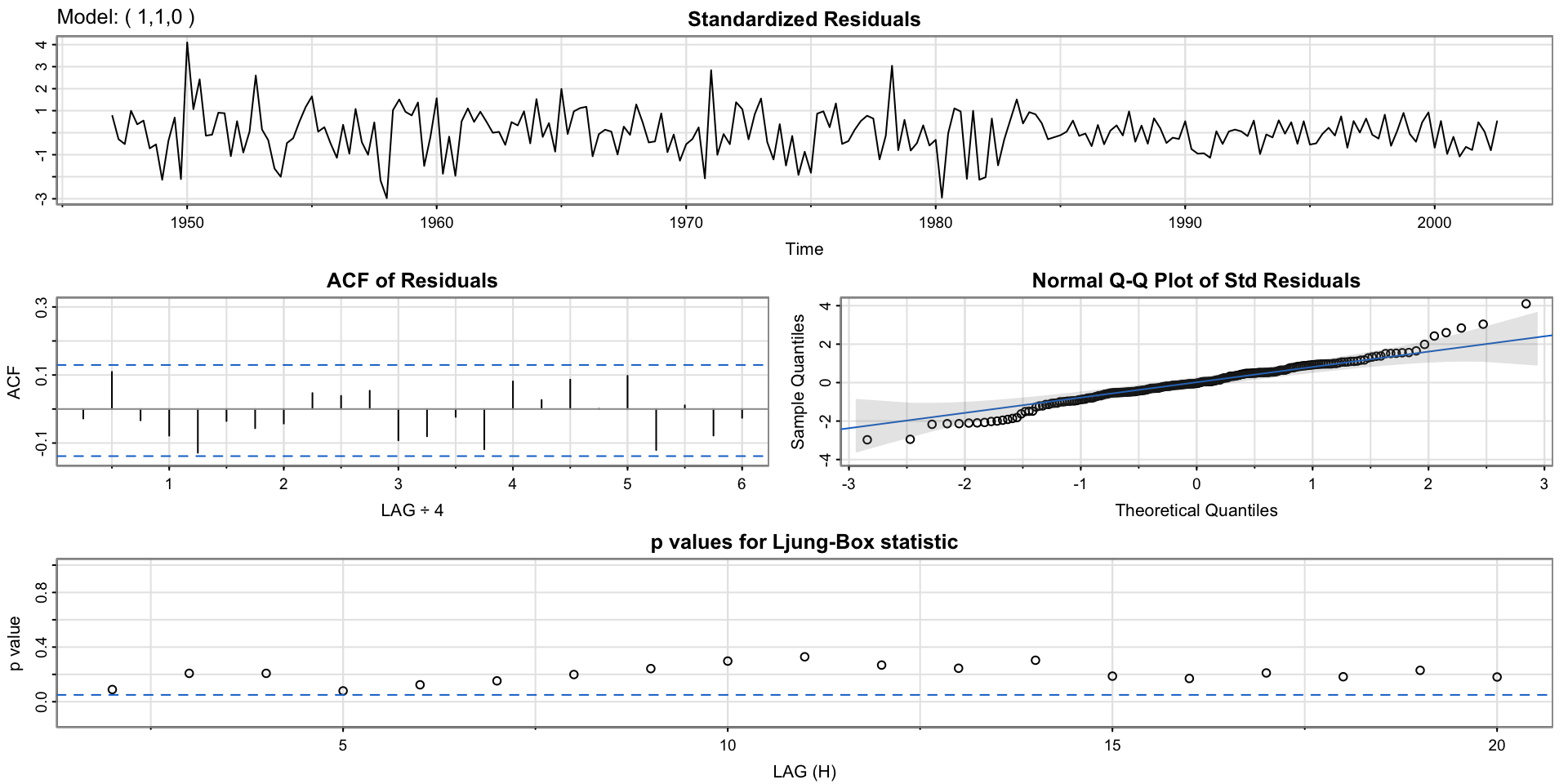
More on the Ljung-box statistic
“another way to view the ACF of the residuals”
“not a bunch of highly dependent tests”
“accumulation of autocorrelation”
“considers the magnitudes” of the autocorrelations all together
\[
Q = n(n+2) + \sum_{h=1}^H \frac{\hat{\rho}_{resid}(h)^2}{n-h}
\] Test statistic used to calcualte p-values in the sarima output– the \(\hat{\rho}_{resid}(h)\) is the sample acf we plot using acf or acf1.
ETS Models
Stepping away from ARIMA for the time being…
Smoothing
We have seen several smoothers:
Moving Average
Loess
Kernel
We have also seen the decompose function, but emphasized it is an exploratory data analysis tool.
What if we wanted to use these equations for forecasting?
Simple exponential smoothing
useful for forecasting data with no trend or seasonal component
Predicts the future as a weighted average of the past, where the weights decrease exponentially the further back in time you go
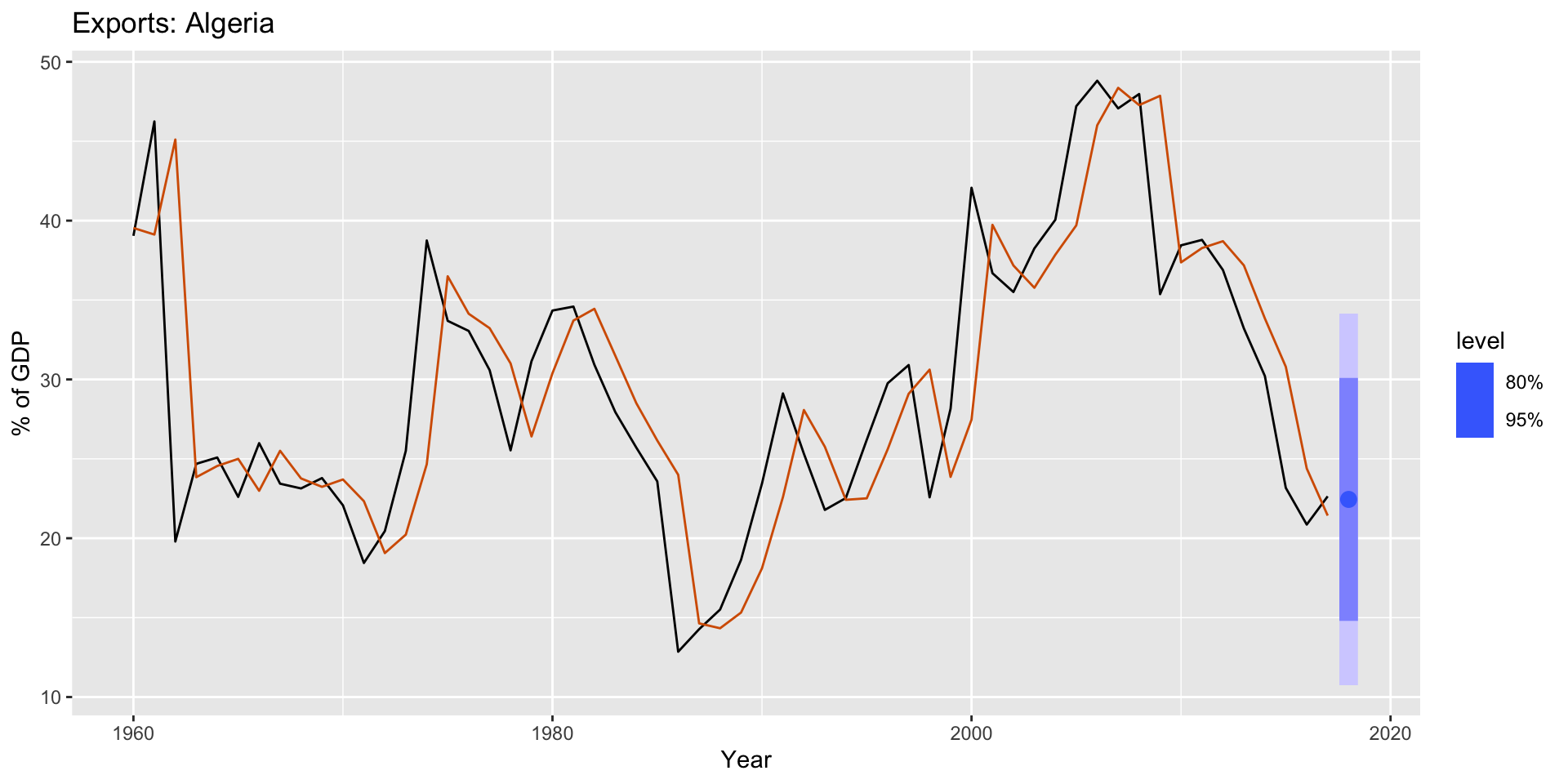
Example: Algerian Exports (FPP 8.1)
Code
algeria_economy <- global_economy |>filter(Country =="Algeria")algeria_economy |>autoplot(Exports) +labs(y ="% of GDP", title ="Exports: Algeria")
the weights are the coefficients in front of the \(y_{T-h}\) terms.
Forecast equation (weighted average form)
We can rewrite the equation as:
\[
\hat{y}_{T+1|T} = \alpha y_T + (1-\alpha) \hat{y}_{T|T-1},
\] In order to forecast the next point, we need to just keep track of the data for the last time point, and the forecast for the last time point.
Easy to update as new data comes in!
Forecast equation (component form)
More notation, but essentially the same thing as the last slide. This representation will be helpful later on.