1  PARE model

1.1 Load data, functions, and packages

Code

library(dplyr)
library(sf)
library(spdep)
library(extRemes)
library(ggplot2)
library(patchwork)

thresh = 253

stations <- read.csv("Data/station_info.csv")
stat_nos <- stations[,1]

source("Code/HelperFunctions_PARE/format_data.R")
source("Code/HelperFunctions_PARE/jitter_n_sym.R")
source("Code/HelperFunctions_PARE/get_sym_car_mat.R")
source("Code/HelperFunctions_PARE/get_par_car.R")
source("Code/HelperFunctions_PARE/get_se.R")
source("Code/HelperFunctions_PARE/pars_to_rl.R")
source("Code/HelperFunctions_PARE/rl_with_ci.R")
source("Code/HelperFunctions_PARE/make_varcov_mats_car.R")
source("Code/HelperFunctions_PARE/rl_ci_to_plot_vec.R")
source("Code/HelperFunctions_PARE/create_mat.R")
source("Code/HelperFunctions_PARE/win_rl_to_plot_dat.R")
source("Code/HelperFunctions_PARE/get_latex_table.R")

1.2 Format time series of GPD fits

## load watershed data
ws_regs <- sf::read_sf("Data/watershed_region_updated")
st_crs(ws_regs) <-sf::st_crs(2278)

## window object generated in Fit_GPD.qmd
## Load rolling GPD fits (takes a bit)
window <- readRDS("Data/window_1day_dclust_updated.rds")  # list of lists (82 x 601) of GPD fits
window_CVM <- readRDS("Data/window_CVM_updated.rds")
window_AD <- readRDS("Data/window_AD_updated.rds")

## Extract windows (note varying # stations)
dat_win_22 <- format_data(window[[22]], stations, ws_regs, window_CVM[[22]]) # 34
dat_win_52 <- format_data(window[[52]], stations, ws_regs, window_CVM[[52]]) # 28
dat_win_82 <- format_data(window[[82]], stations, ws_regs, window_CVM[[82]]) # 149

## save values (faster than reading entire window[[]] object)
save(dat_win_22, file = "Data/dat_win_22")
save(dat_win_52, file = "Data/dat_win_52")
save(dat_win_82, file = "Data/dat_win_82")

1.3 Construct spatial weight matrices

Generating the Hausdorff matrix

The hausMat function and additional documentation can be found in the hausdorff Github repository.

# (make sure ws_regs is projected first)
distMat <- hausMat(ws_regs, f1 = 0.5)
distMat/5280

# save output
# saveRDS(distMat, file = "~/Documents/GitHub/Spatial_Extreme_Value_Modeling/Data/hMat_med.rds")

# read in previously computed Hausdorff matrix and convert units to miles
hMat <- readRDS(file = "Data/hMat_med.rds")
hMat_miles <- hMat/5280

## Create weight matrix for each window 
## Accounts for different numbers of stations (varying point-to-area structure)
## Jiters the values to give valid weight matrix
set.seed(24)
D_22 <- get_sym_car_mat(dat_win_22, hMat_miles)
D_52 <- get_sym_car_mat(dat_win_52, hMat_miles)
D_82 <- get_sym_car_mat(dat_win_82, hMat_miles)

1.4 Fit models to each window for each parameter

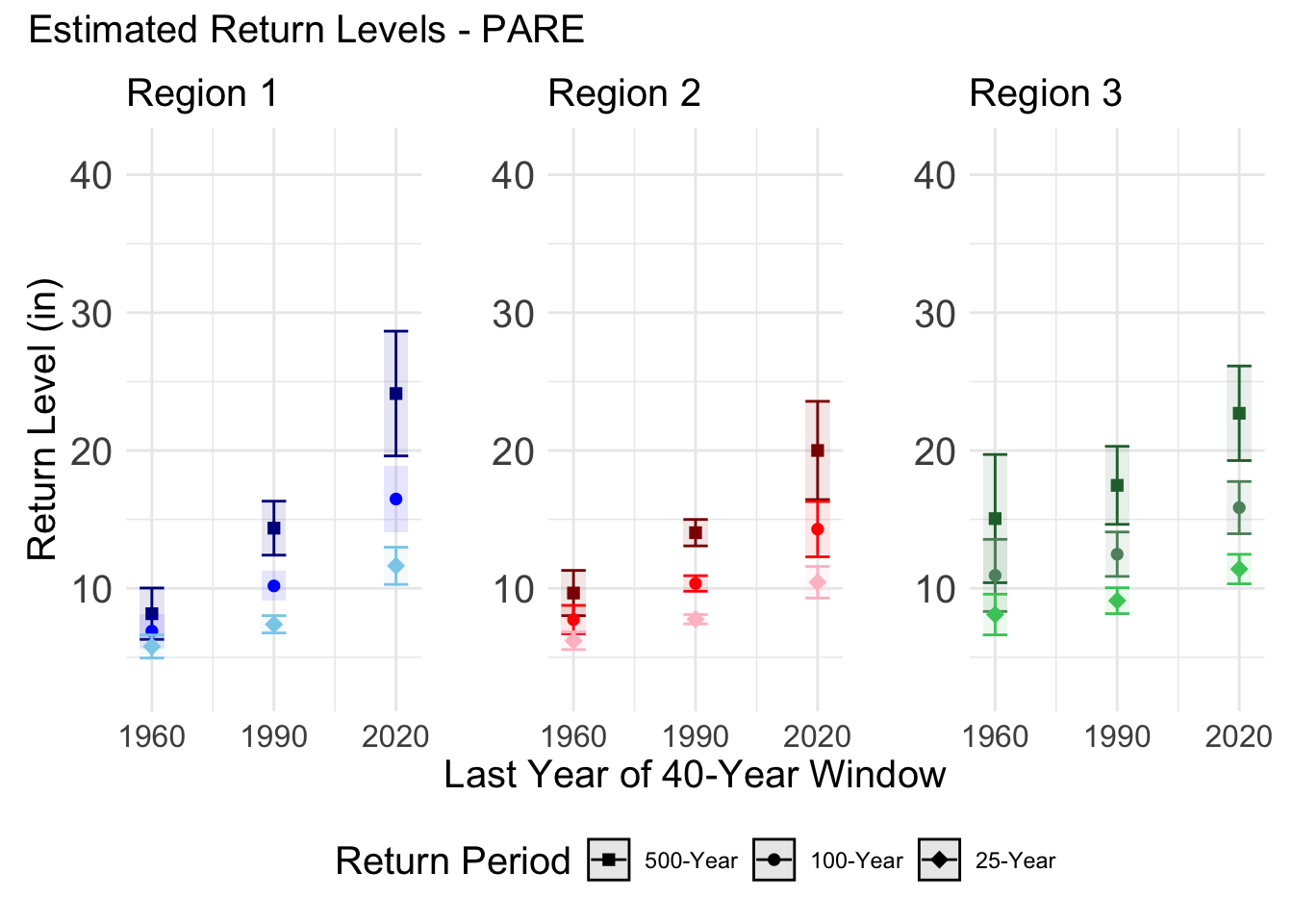
To obtain region-level estimates of the GPD parameters, fit a conditional auto-regressive model for each GPD parameter for each window, a total of 9 models.

## window 22
## Fit models
car_shape_22 <- spatialreg::spautolm(shape ~ -1 + Reg1 + Reg2 + Reg3, 
                                     data = dat_win_22, family="CAR", 
                                     listw=mat2listw(1/D_22, style = "C"))
car_ln.scale_22 <- spatialreg::spautolm(log(scale) ~ -1 + Reg1 + Reg2 + Reg3, 
                                        data = dat_win_22, family="CAR", 
                                        listw=mat2listw(1/D_22,style = "C"))
car_rate_22 <- spatialreg::spautolm(rate ~ -1 + Reg1 + Reg2 + Reg3, 
                                    data = dat_win_22, family="CAR", 
                                    listw=mat2listw(1/D_22, style = "C"))
## extract parameter estimates
par_22 <- get_par_car(car_ln.scale_22, car_shape_22, car_rate_22)
se_22 <- get_se(car_ln.scale_22, car_shape_22, car_rate_22)[3,]
car_varcov_22 <- make_varcov_mats_car(car_ln.scale_22, car_shape_22)  # se of scale 8.5, 4, 9.25
st_devs_22 <- data.frame(Reg1 = c(sqrt(diag(car_varcov_22[[1]])), se_22[1]),
                         Reg2 = c(sqrt(diag(car_varcov_22[[2]])), se_22[2]), 
                         Reg3 = c(sqrt(diag(car_varcov_22[[3]])), se_22[3]))
row.names(st_devs_22) <- row.names(par_22)



## window 52
## Fit models
car_shape_52 <- spatialreg::spautolm(shape ~ -1 + Reg1 + Reg2 + Reg3, 
                                     data = dat_win_52, family="CAR", 
                                     listw=mat2listw(1/D_52, style = "C"))
car_ln.scale_52 <- spatialreg::spautolm(log(scale) ~ -1 + Reg1 + Reg2 + Reg3, 
                                        data = dat_win_52, family="CAR", 
                                        listw=mat2listw(1/D_52, style = "C"))
car_rate_52 <- spatialreg::spautolm(rate ~ -1 + Reg1 + Reg2 + Reg3, 
                                    data = dat_win_52, family="CAR", 
                                    listw=mat2listw(1/D_52, style = "C"))
## Extract parameter estimates
par_52 <- get_par_car(car_ln.scale_52, car_shape_52, car_rate_52)
se_52 <- get_se(car_ln.scale_52, car_shape_52, car_rate_52)[3,]
car_varcov_52 <- make_varcov_mats_car(car_ln.scale_52, car_shape_52)  # se of scale 8.5, 4, 9.25
st_devs_52 <- data.frame(Reg1 = c(sqrt(diag(car_varcov_52[[1]])), se_52[1]),
                         Reg2 = c(sqrt(diag(car_varcov_52[[2]])), se_52[2]), 
                         Reg3 = c(sqrt(diag(car_varcov_52[[3]])), se_52[3]))

## window 82
## fit models
car_shape_82 <- spatialreg::spautolm(shape ~ -1 + Reg1 + Reg2 + Reg3, 
                                     data = dat_win_82, family="CAR", 
                                     listw=mat2listw(1/D_82, style = "C"))
car_ln.scale_82 <- spatialreg::spautolm(log(scale) ~ -1 + Reg1 + Reg2 + Reg3, 
                                        data = dat_win_82, family="CAR", 
                                        listw=mat2listw(1/D_82, style = "C"))
car_rate_82 <- spatialreg::spautolm(rate ~ -1 + Reg1 + Reg2 + Reg3, 
                                    data = dat_win_82, family="CAR", 
                                    listw=mat2listw(1/D_82, style = "C"))
## Extract parameter estiamtes
par_82 <- get_par_car(car_ln.scale_82, car_shape_82, car_rate_82)
se_82 <- get_se(car_ln.scale_82, car_shape_82, car_rate_82)[3,]
car_varcov_82 <- make_varcov_mats_car(car_ln.scale_82, car_shape_82)  # se of scale 8.5, 4, 9.25
st_devs_82 <- data.frame(Reg1 = c(sqrt(diag(car_varcov_82[[1]])), se_82[1]),
                         Reg2 = c(sqrt(diag(car_varcov_82[[2]])), se_82[2]), 
                         Reg3 = c(sqrt(diag(car_varcov_82[[3]])), se_82[3]))

1.4.1 Table of parameter estimates

PARE portion of Table S3 
 First 40 Years of Data (1921-1960) 
 Parameters

              Reg1         Reg2         Reg3
scale 230.85855709 200.15626351 198.45979895
shape  -0.01912063   0.05329551   0.14923817
rate    0.02814622   0.03138875   0.03426008

Standard Errors

              Reg1         Reg2         Reg3
scale 5.3213141641 3.0221032578 4.5999740852
shape 0.0313947823 0.0204812334 0.0315739476
rate  0.0005872697 0.0003877783 0.0005903755

PARE portion of Table S4 
 Second 40 Years of Data (1951-1990) 
 Parameters

              Reg1        Reg2         Reg3
scale 171.95531347 202.3189569 217.80371166
shape   0.17232481   0.1340430   0.16194601
rate    0.02981064   0.0317399   0.03388214

Standard Errors

          Reg1         Reg2         Reg3
1 4.4827004098 2.7176004289 6.6253934853
2 0.0131459688 0.0067930158 0.0153266095
3 0.0006522969 0.0003391368 0.0007591396

PARE portion of Table 2 
 Last 40 Years of Data (1981-2020) 
 Parameters

              Reg1         Reg2         Reg3
scale 215.07848444 236.68456472 223.98647292
shape   0.20456458   0.16327472   0.18610913
rate    0.05510062   0.04333857   0.05629901

Standard Errors

         Reg1        Reg2        Reg3
1 4.323191117 4.894934005 3.699432968
2 0.016361116 0.016841085 0.013420937
3 0.002272369 0.002339033 0.001864008

1.5 Calculate return levels + CIs

### Estimates and CIs for visuals
car_rl_25_22  <- rl_with_ci(par_mat = par_22, 
                            varcov_list = car_varcov_22, 
                            return_period = 25, 
                            type = "ci", alpha = 0.05)/254
car_rl_100_22 <- rl_with_ci(par_22, car_varcov_22, 100, "ci")/254
car_rl_500_22 <- rl_with_ci(par_22, car_varcov_22, 500, "ci")/254

car_rl_25_52  <- rl_with_ci(par_52, car_varcov_52, 25, "ci")/254
car_rl_100_52 <- rl_with_ci(par_52, car_varcov_52, 100, "ci")/254
car_rl_500_52 <- rl_with_ci(par_52, car_varcov_52, 500, "ci")/254

car_rl_25_82  <- rl_with_ci(par_82, car_varcov_82, 25, "ci")/254
car_rl_100_82 <- rl_with_ci(par_82, car_varcov_82, 100, "ci")/254
car_rl_500_82 <- rl_with_ci(par_82, car_varcov_82, 500, "ci")/254

win_1 <- rl_ci_to_plot_vec(car_rl_25_22, car_rl_100_22, car_rl_500_22)
win_2 <- rl_ci_to_plot_vec(car_rl_25_52, car_rl_100_52, car_rl_500_52)
win_3 <- rl_ci_to_plot_vec(car_rl_25_82, car_rl_100_82, car_rl_500_82)

plot_dat <- win_rl_to_plot_dat(win_1, win_2, win_3)
reg1 <- plot_dat[[1]] # Region 1 data frame for plotting
reg2 <- plot_dat[[2]] 
reg3 <- plot_dat[[3]] 

1.5.1 Visualizations

## define horizontal limits for error bars
reg1$LB_X <- reg2$LB_X <- reg3$LB_X <- c(1957, 1987, 2017)
reg1$UB_X <- reg2$UB_X <- reg3$UB_X <- c(1963, 1993, 2023)

## legend 
g <- guides(fill = guide_legend(override.aes = list(color = c("black", "black", "black"),
                                                    shape = c(15, 16, 18), 
                                                    fill = c("black", "black", "black"),
                                                    linetype = c(1,1,1),
                                                    size = c(2,2,3)
                                                    )))

## Region 1
reg1_plot <- ggplot(data=reg1, aes(x=c(1960, 1990, 2020))) + 
    coord_cartesian(ylim = c(3, 41.5)) +
  ## 500 year
    geom_point(aes(y=RL_500, color="500-Year", shape = "500-Year"), size = 2) + 
    geom_errorbar(aes(ymin=LB_500, ymax=UB_500, col="500-Year", linetype = "500-Year"), width = 6)+ 
    geom_rect(aes(ymin=LB_500, ymax=UB_500,xmin = LB_X, xmax = UB_X, fill="500-Year"), alpha=0.1)+
  ## 100 year
    geom_point(aes(y=RL_100, color="100-Year", shape = "100-Year"), size = 2)+ 
    #geom_errorbar(aes(ymin=LB_100, ymax=UB_100, col="100-Year", linetype = "100-Year"), width = 6) +     
    geom_rect(aes(ymin=LB_100, ymax=UB_100,xmin = LB_X, xmax = UB_X, fill="100-Year"), alpha=0.1)+
  ##25 year
    geom_point(aes(y=RL_25, color="25-Year", shape = "25-Year"), size = 3) + 
    geom_errorbar(aes(ymin=LB_25, ymax=UB_25, col="25-Year", linetype = "25-Year"), width = 6) +
    geom_rect(aes(ymin=LB_25, ymax=UB_25,xmin = LB_X, xmax = UB_X, fill="25-Year"), alpha=0.1)+
    scale_x_continuous(breaks = c(1960, 1990,2020)) +
    scale_colour_manual(name = "Return Period", 
                        values = c('500-Year' = "darkblue", '100-Year' = "blue", '25-Year' = "skyblue"),
                        breaks = c('500-Year', '100-Year', '25-Year')) + 
    scale_linetype_manual(values = c("500-Year" = "solid", "100-Year" = "solid", "25-Year" = "solid"),
                          breaks = c('500-Year', '100-Year', '25-Year'), name = "Return Period") +
  scale_fill_manual(name = "Return Period", values =  c('500-Year' = "darkblue", '100-Year' = "blue", '25-Year' = "lightblue"), breaks = c('500-Year', '100-Year', '25-Year'))+
    scale_shape_manual(name = "Return Period", values = c('500-Year' = 15, '100-Year' = 16, '25-Year' = 18), breaks = c('500-Year', '100-Year', '25-Year')) +
     labs(x="", y="Return Level (in)", title="Region 1") + theme_minimal() +   theme(legend.position="none",  
        axis.text.y = element_text(size = 15), 
        axis.text.x = element_text(size = 12), 
        axis.title.x = element_text(size = 15), 
        title = element_text(size = 15))

## Region 2
reg2_plot <- ggplot(data=reg2, aes(x=c(1960, 1990, 2020))) + 
    coord_cartesian(ylim = c(3, 41.5)) +
  ## 500 year
    geom_point(aes(y=RL_500, color="500-Year", shape = "500-Year"), size = 2) + 
    geom_errorbar(aes(ymin=LB_500, ymax=UB_500, col="500-Year", linetype = "500-Year"), width = 6)+ 
    geom_rect(aes(ymin=LB_500, ymax=UB_500,xmin = LB_X, xmax = UB_X, fill="500-Year"), alpha=0.1)+
  ## 100 year
    geom_point(aes(y=RL_100, color="100-Year", shape = "100-Year"), size = 2)+ 
    geom_errorbar(aes(ymin=LB_100, ymax=UB_100, col="100-Year", linetype = "100-Year"), width = 6) +     
    geom_rect(aes(ymin=LB_100, ymax=UB_100,xmin = LB_X, xmax = UB_X, fill="100-Year"), alpha=0.1)+
  ##25 year
    geom_point(aes(y=RL_25, color="25-Year", shape = "25-Year"), size = 3) + 
    geom_errorbar(aes(ymin=LB_25, ymax=UB_25, col="25-Year", linetype = "25-Year"), width = 6) +
    geom_rect(aes(ymin=LB_25, ymax=UB_25,xmin = LB_X, xmax = UB_X, fill="25-Year"), alpha=0.1)+
    scale_x_continuous(breaks = c(1960, 1990,2020)) +
    scale_colour_manual(name = "Return Period", 
                        values = c('500-Year' = "darkred", '100-Year' = "red", '25-Year' = "pink"),
                        breaks = c('500-Year', '100-Year', '25-Year')) + 
    scale_linetype_manual(values = c("500-Year" = "solid", "100-Year" = "solid", "25-Year" = "solid"),
                          breaks = c('500-Year', '100-Year', '25-Year'), name = "Return Period") +
  scale_fill_manual(name = "Return Period", values =  c('500-Year' = "darkred", '100-Year' = "red", '25-Year' = "pink"), breaks = c('500-Year', '100-Year', '25-Year'))+
    scale_shape_manual(name = "Return Period", values = c('500-Year' = 15, '100-Year' = 16, '25-Year' = 18), breaks = c('500-Year', '100-Year', '25-Year')) +
     labs(x="Last Year of 40-Year Window", y="", title="Region 2") + theme_minimal() + g +   theme(legend.position="bottom",  
        axis.text.y = element_text(size = 15), 
        axis.text.x = element_text(size = 12), 
        axis.title.x = element_text(size = 15), 
        title = element_text(size = 15))



## Region 3
reg3_plot <- ggplot(data=reg3, aes(x=c(1960, 1990, 2020))) + 
    coord_cartesian(ylim = c(3, 41.5)) +
  ## 500 year
    geom_point(aes(y=RL_500, color="500-Year", shape = "500-Year"), size = 2) + 
    geom_errorbar(aes(ymin=LB_500, ymax=UB_500, col="500-Year", linetype = "500-Year"), width = 6)+ 
    geom_rect(aes(ymin=LB_500, ymax=UB_500,xmin = LB_X, xmax = UB_X, fill="500-Year"), alpha=0.1)+
  ## 100 year
    geom_point(aes(y=RL_100, color="100-Year", shape = "100-Year"), size = 2)+ 
    geom_errorbar(aes(ymin=LB_100, ymax=UB_100, col="100-Year", linetype = "100-Year"), width = 6) +     
    geom_rect(aes(ymin=LB_100, ymax=UB_100,xmin = LB_X, xmax = UB_X, fill="100-Year"), alpha=0.1)+
  ##25 year
    geom_point(aes(y=RL_25, color="25-Year", shape = "25-Year"), size = 3) + 
    geom_errorbar(aes(ymin=LB_25, ymax=UB_25, col="25-Year", linetype = "25-Year"), width = 6) +
    geom_rect(aes(ymin=LB_25, ymax=UB_25,xmin = LB_X, xmax = UB_X, fill="25-Year"), alpha=0.1)+
    scale_x_continuous(breaks = c(1960, 1990,2020)) +
    scale_colour_manual(name = "Return Period", 
                        values = c('500-Year' = "#256e3a", '100-Year' = "#5d916c", '25-Year' = "#44c96a"),
                        breaks = c('500-Year', '100-Year', '25-Year')) + 
    scale_linetype_manual(values = c("500-Year" = "solid", "100-Year" = "solid", "25-Year" = "solid"),
                          breaks = c('500-Year', '100-Year', '25-Year'), name = "Return Period") +
  scale_fill_manual(name = "Return Period", values =  c('500-Year' = "#256e3a", '100-Year' = "#5d916c", '25-Year' = "#44c96a"), breaks = c('500-Year', '100-Year', '25-Year'))+
    scale_shape_manual(name = "Return Period", values = c('500-Year' = 15, '100-Year' = 16, '25-Year' = 18), breaks = c('500-Year', '100-Year', '25-Year')) +
     labs(x="", y="", title="Region 3") + theme_minimal() + 
    theme(legend.position="none",  
        axis.text.y = element_text(size = 15), 
        axis.text.x = element_text(size = 12), 
        axis.title.x = element_text(size = 15), 
        title = element_text(size = 15))





PARE_plot = reg1_plot + reg2_plot + reg3_plot +plot_layout(ncol = 3) + 
  plot_annotation("Estimated Return Levels - PARE") & theme(plot.title = element_text(size = 15))

#ggsave("Images/PARE_plot.png", plot = PARE_plot, width = 7.5, height = 3.5, units = "in")

PARE_plot

1.5.2 Table of return levels

## Table S3
car_rl_25_22_se  <- rl_with_ci(par_mat = par_22, 
                            varcov_list = car_varcov_22, 
                            return_period = 25, 
                            type = "se", alpha = 0.05)/254
car_rl_100_22_se <- rl_with_ci(par_22, car_varcov_22, 100, "se")/254
car_rl_500_22_se <- rl_with_ci(par_22, car_varcov_22, 500, "se")/254

print("Return Levels for First 40 Years of Data (1921-1960)")

[1] "Return Levels for First 40 Years of Data (1921-1960)"

rbind(t(car_rl_25_22_se), t(car_rl_100_22_se), t(car_rl_500_22_se))

               Reg1      Reg2       Reg3
25-yr RL  5.7812602 6.2000477  8.1017057
SE        0.4268857 0.3273666  0.7538876
100-yr RL 6.8995253 7.7328867 10.9382561
SE        0.6450349 0.5268412  1.3344426
500-yr RL 8.1611487 9.6604967 15.0588530
SE        0.9508076 0.8372663  2.3736257

## latex output
# car_rl_22_list <- list(car_rl_25_22_se, car_rl_100_22_se, car_rl_500_22_se)
# get_latex_table_RL(car_rl_22_list)


## Table S4
car_rl_25_52_se  <- rl_with_ci(par_52, car_varcov_52, 25, "se")/254
car_rl_100_52_se <- rl_with_ci(par_52, car_varcov_52, 100, "se")/254
car_rl_500_52_se <- rl_with_ci(par_52, car_varcov_52, 500, "se")/254

print("Return Levels for Second 40 Years of Data (1951-1990)")

[1] "Return Levels for Second 40 Years of Data (1951-1990)"

rbind(t(car_rl_25_52_se), t(car_rl_100_52_se), t(car_rl_500_52_se))

                Reg1       Reg2       Reg3
25-yr RL   7.3910220  7.7591772  9.1036876
SE         0.3201394  0.1732745  0.4792676
100-yr RL 10.1767483 10.3537503 12.4771511
SE         0.5586972  0.2883097  0.8222935
500-yr RL 14.3667665 14.0375739 17.4724334
SE         0.9991024  0.4890933  1.4436359

# Latex output
# car_rl_52_list <- list(car_rl_25_52_se, car_rl_100_52_se, car_rl_500_52_se)
# get_latex_table_RL(car_rl_52_list)


## TABLE S2 (also Table 3)
car_rl_25_82_se  <- rl_with_ci(par_82, car_varcov_82, 25, "se")/254
car_rl_100_82_se <- rl_with_ci(par_82, car_varcov_82, 100, "se")/254
car_rl_500_82_se <- rl_with_ci(par_82, car_varcov_82, 500, "se")/254

# Latex output
# car_rl_82_list <- list(car_rl_25_82_se, car_rl_100_82_se, car_rl_500_82_se)
# get_latex_table_RL(car_rl_82_list)
print("Return Levels for First 40 Years of Data (1981-2020)")

[1] "Return Levels for First 40 Years of Data (1981-2020)"

rbind(t(car_rl_25_82_se), t(car_rl_100_82_se), t(car_rl_500_82_se))

               Reg1       Reg2       Reg3
25-yr RL  11.634249 10.4422599 11.3992557
SE         0.687375  0.5856544  0.5461398
100-yr RL 16.479569 14.2913625 15.8560177
SE         1.243511  1.0239274  0.9666489
500-yr RL 24.130583 20.0023744 22.7002292
SE         2.309727  1.8186076  1.7503930

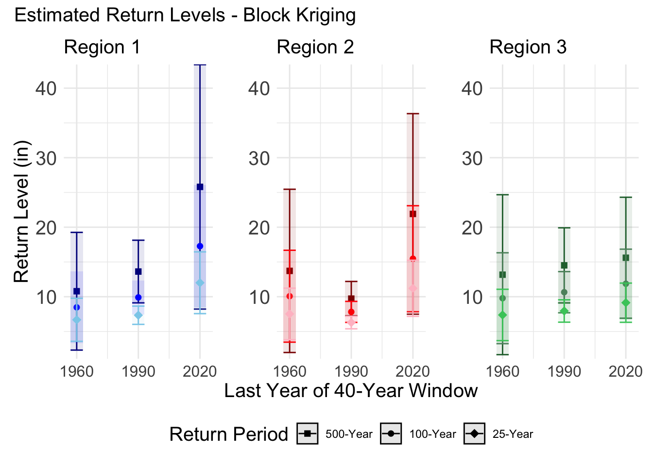
1.6 Block Kriging

Data for Block Kriging Return Level plots from Fagnant ’21 (Block Kriging sections of Tables 5.3, 5.6, 5.7). Data also included in manuscript in Block Kriging section of Tables S5, S6, S2, and 3.

## read in values for Block Kriging-- read from Fagnant 2021
reg1_bk <- data.frame(RL_25 = c(6.681,7.337,12.008), 
                   RL_100 = c(8.472,9.900,17.277), 
                   RL_500 = c(10.789,13.621,25.800))
reg1_bk$LB_25 = reg1_bk$RL_25 - 1.96*c(1.578,0.670,2.266)
reg1_bk$UB_25 = reg1_bk$RL_25 + 1.96*c(1.578,0.670,2.266)

reg1_bk$LB_100 = reg1_bk$RL_100 - 1.96*c(2.630,1.244,4.485)
reg1_bk$UB_100 = reg1_bk$RL_100 + 1.96*c(2.630,1.244,4.485)

reg1_bk$LB_500 = reg1_bk$RL_500 - 1.96*c(4.319, 2.299,8.969)
reg1_bk$UB_500 = reg1_bk$RL_500 + 1.96*c(4.319, 2.299,8.969)

reg1_bk$LB_X <- c(1957, 1987, 2017)
reg1_bk$UB_X <- c(1963, 1993, 2023)

reg2_bk <- data.frame(RL_25 = c(7.523,6.289,11.210), 
                   RL_100 = c(10.073,7.818,15.465), 
                   RL_500 = c(13.717,9.728,21.911))

reg2_bk$LB_25 = reg2_bk$RL_25 - 1.96*c(1.895, 0.462, 2.06)
reg2_bk$UB_25 = reg2_bk$RL_25 + 1.96*c(1.895, 0.462, 2.06)

reg2_bk$LB_100 = reg2_bk$RL_100 - 1.96*c(3.372,0.771,3.89)
reg2_bk$UB_100 = reg2_bk$RL_100 + 1.96*c(3.372,0.771,3.89)

reg2_bk$LB_500 = reg2_bk$RL_500 - 1.96*c(5.990, 1.260,7.36)
reg2_bk$UB_500 = reg2_bk$RL_500 + 1.96*c(5.990, 1.260,7.36)

reg2_bk$LB_X <- c(1957, 1987, 2017)
reg2_bk$UB_X <- c(1963, 1993, 2023)


reg3_bk <- data.frame(RL_25 = c(7.376,7.950,9.141), 
                   RL_100 = c(9.784,10.650,11.865), 
                   RL_500 = c(13.170,14.511,15.607))

reg3_bk$LB_25 = reg3_bk$RL_25 - 1.96*c(1.885,0.823, 1.44)
reg3_bk$UB_25 = reg3_bk$RL_25 + 1.96*c(1.885,0.823, 1.44)

reg3_bk$LB_100 = reg3_bk$RL_100 - 1.96*c(3.335,1.511, 2.54)
reg3_bk$UB_100 = reg3_bk$RL_100 + 1.96*c(3.335,1.511, 2.54)

reg3_bk$LB_500 = reg3_bk$RL_500 - 1.96*c(5.870,2.757,4.44)
reg3_bk$UB_500 = reg3_bk$RL_500 + 1.96*c(5.870,2.757,4.44)

reg3_bk$LB_X <- c(1957, 1987, 2017)
reg3_bk$UB_X <- c(1963, 1993, 2023)

1.6.1 Visualizations

## legend 
g <- guides(fill = guide_legend(override.aes = list(color = c("black", "black", "black"),
                                                    shape = c(15, 16, 18), 
                                                    fill = c("black", "black", "black"),
                                                    linetype = c(1,1,1),
                                                    size = c(2,2,3)
                                                    )))

## Region 1
reg1_bk_plot <- ggplot(data=reg1_bk, aes(x=c(1960, 1990, 2020))) + 
    coord_cartesian(ylim = c(3, 41.5)) +
  ## 500 year
    geom_point(aes(y=RL_500, color="500-Year", shape = "500-Year"), size = 2) + 
    geom_errorbar(aes(ymin=LB_500, ymax=UB_500, col="500-Year", linetype = "500-Year"), width = 6)+ 
    geom_rect(aes(ymin=LB_500, ymax=UB_500,xmin = LB_X, xmax = UB_X, fill="500-Year"), alpha=0.1)+
  ## 100 year
    geom_point(aes(y=RL_100, color="100-Year", shape = "100-Year"), size = 2)+ 
    #geom_errorbar(aes(ymin=LB_100, ymax=UB_100, col="100-Year", linetype = "100-Year"), width = 6) +     
    geom_rect(aes(ymin=LB_100, ymax=UB_100,xmin = LB_X, xmax = UB_X, fill="100-Year"), alpha=0.1)+
  ##25 year
    geom_point(aes(y=RL_25, color="25-Year", shape = "25-Year"), size = 3) + 
    geom_errorbar(aes(ymin=LB_25, ymax=UB_25, col="25-Year", linetype = "25-Year"), width = 6) +
    geom_rect(aes(ymin=LB_25, ymax=UB_25,xmin = LB_X, xmax = UB_X, fill="25-Year"), alpha=0.1)+
    scale_x_continuous(breaks = c(1960, 1990,2020)) +
    scale_colour_manual(name = "Return Period", 
                        values = c('500-Year' = "darkblue", '100-Year' = "blue", '25-Year' = "skyblue"),
                        breaks = c('500-Year', '100-Year', '25-Year')) + 
    scale_linetype_manual(values = c("500-Year" = "solid", "100-Year" = "solid", "25-Year" = "solid"),
                          breaks = c('500-Year', '100-Year', '25-Year'), name = "Return Period") +
  scale_fill_manual(name = "Return Period", values =  c('500-Year' = "darkblue", '100-Year' = "blue", '25-Year' = "lightblue"), breaks = c('500-Year', '100-Year', '25-Year'))+
    scale_shape_manual(name = "Return Period", values = c('500-Year' = 15, '100-Year' = 16, '25-Year' = 18), breaks = c('500-Year', '100-Year', '25-Year')) +
     labs(x="", y="Return Level (in)", title="Region 1") + theme_minimal() +   theme(legend.position="none",  
        axis.text.y = element_text(size = 15), 
        axis.text.x = element_text(size = 12), 
        axis.title.x = element_text(size = 15), 
        title = element_text(size = 15))


## Region 2
reg2_bk_plot <- ggplot(data=reg2_bk, aes(x=c(1960, 1990, 2020))) + 
    coord_cartesian(ylim = c(3, 41.5)) +
  ## 500 year
    geom_point(aes(y=RL_500, color="500-Year", shape = "500-Year"), size = 2) + 
    geom_errorbar(aes(ymin=LB_500, ymax=UB_500, col="500-Year", linetype = "500-Year"), width = 6)+ 
    geom_rect(aes(ymin=LB_500, ymax=UB_500,xmin = LB_X, xmax = UB_X, fill="500-Year"), alpha=0.1)+
  ## 100 year
    geom_point(aes(y=RL_100, color="100-Year", shape = "100-Year"), size = 2)+ 
    geom_errorbar(aes(ymin=LB_100, ymax=UB_100, col="100-Year", linetype = "100-Year"), width = 6) +     
    geom_rect(aes(ymin=LB_100, ymax=UB_100,xmin = LB_X, xmax = UB_X, fill="100-Year"), alpha=0.1)+
  ##25 year
    geom_point(aes(y=RL_25, color="25-Year", shape = "25-Year"), size = 3) + 
    geom_errorbar(aes(ymin=LB_25, ymax=UB_25, col="25-Year", linetype = "25-Year"), width = 6) +
    geom_rect(aes(ymin=LB_25, ymax=UB_25,xmin = LB_X, xmax = UB_X, fill="25-Year"), alpha=0.1)+
    scale_x_continuous(breaks = c(1960, 1990,2020)) +
    scale_colour_manual(name = "Return Period", 
                        values = c('500-Year' = "darkred", '100-Year' = "red", '25-Year' = "pink"),
                        breaks = c('500-Year', '100-Year', '25-Year')) + 
    scale_linetype_manual(values = c("500-Year" = "solid", "100-Year" = "solid", "25-Year" = "solid"),
                          breaks = c('500-Year', '100-Year', '25-Year'), name = "Return Period") +
  scale_fill_manual(name = "Return Period", values =  c('500-Year' = "darkred", '100-Year' = "red", '25-Year' = "pink"), breaks = c('500-Year', '100-Year', '25-Year'))+
    scale_shape_manual(name = "Return Period", values = c('500-Year' = 15, '100-Year' = 16, '25-Year' = 18), breaks = c('500-Year', '100-Year', '25-Year')) +
     labs(x="Last Year of 40-Year Window", y="", title="Region 2") + theme_minimal() + g +   theme(legend.position="bottom",  
        axis.text.y = element_text(size = 15), 
        axis.text.x = element_text(size = 12), 
        axis.title.x = element_text(size = 15), 
        title = element_text(size = 15))



## Region 3
reg3_bk_plot <- ggplot(data=reg3_bk, aes(x=c(1960, 1990, 2020))) + 
    coord_cartesian(ylim = c(3, 41.5)) +
  ## 500 year
    geom_point(aes(y=RL_500, color="500-Year", shape = "500-Year"), size = 2) + 
    geom_errorbar(aes(ymin=LB_500, ymax=UB_500, col="500-Year", linetype = "500-Year"), width = 6)+ 
    geom_rect(aes(ymin=LB_500, ymax=UB_500,xmin = LB_X, xmax = UB_X, fill="500-Year"), alpha=0.1)+
  ## 100 year
    geom_point(aes(y=RL_100, color="100-Year", shape = "100-Year"), size = 2)+ 
    geom_errorbar(aes(ymin=LB_100, ymax=UB_100, col="100-Year", linetype = "100-Year"), width = 6) +     
    geom_rect(aes(ymin=LB_100, ymax=UB_100,xmin = LB_X, xmax = UB_X, fill="100-Year"), alpha=0.1)+
  ##25 year
    geom_point(aes(y=RL_25, color="25-Year", shape = "25-Year"), size = 3) + 
    geom_errorbar(aes(ymin=LB_25, ymax=UB_25, col="25-Year", linetype = "25-Year"), width = 6) +
    geom_rect(aes(ymin=LB_25, ymax=UB_25,xmin = LB_X, xmax = UB_X, fill="25-Year"), alpha=0.1)+
    scale_x_continuous(breaks = c(1960, 1990,2020)) +
    scale_colour_manual(name = "Return Period", 
                        values = c('500-Year' = "#256e3a", '100-Year' = "#5d916c", '25-Year' = "#44c96a"),
                        breaks = c('500-Year', '100-Year', '25-Year')) + 
    scale_linetype_manual(values = c("500-Year" = "solid", "100-Year" = "solid", "25-Year" = "solid"),
                          breaks = c('500-Year', '100-Year', '25-Year'), name = "Return Period") +
  scale_fill_manual(name = "Return Period", values =  c('500-Year' = "#256e3a", '100-Year' = "#5d916c", '25-Year' = "#44c96a"), breaks = c('500-Year', '100-Year', '25-Year'))+
    scale_shape_manual(name = "Return Period", values = c('500-Year' = 15, '100-Year' = 16, '25-Year' = 18), breaks = c('500-Year', '100-Year', '25-Year')) +
     labs(x="", y="", title="Region 3") + theme_minimal() + 
  theme(legend.position="none",  
        axis.text.y = element_text(size = 15), 
        axis.text.x = element_text(size = 12), 
        axis.title.x = element_text(size = 15), 
        title = element_text(size = 15))





BK_plot = reg1_bk_plot + reg2_bk_plot + reg3_bk_plot +plot_layout(ncol = 3) + plot_annotation("Estimated Return Levels - Block Kriging") & theme(plot.title = element_text(size = 15))

BK_plot

ggsave("Images/BK_plot.png", plot = BK_plot, width = 7.5, height = 3.5, units = "in")

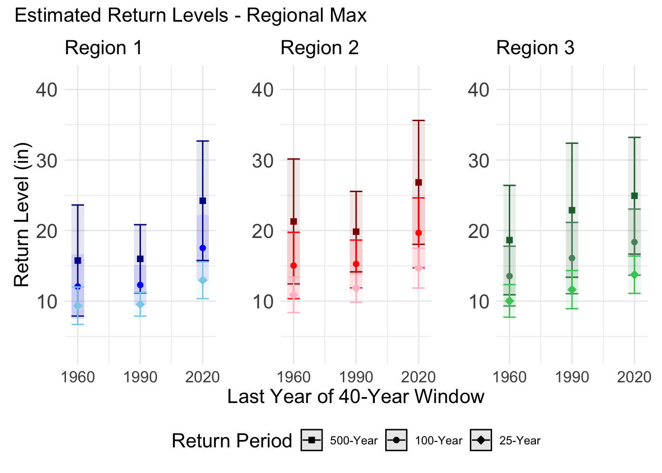
1.7 Regional Max

Data for Regional Max Return Level plots from Fagnant ’21 (Regional Max sections of Tables 5.3, 5.6, 5.7). Data also included in manuscript in Regional Max section of Tables S5, S6, S2, and 3.

## read in values for Regional Max-- read from Fagnant 2021
reg1_rm <- data.frame(RL_25 = c(9.349, 9.552, 12.96), 
                   RL_100 = c(12.073, 12.295, 17.54), 
                   RL_500 = c(15.759, 15.999, 24.23))
reg1_rm$LB_25 = reg1_rm$RL_25 - 1.96*c(1.354, 0.854, 1.33)
reg1_rm$UB_25 = reg1_rm$RL_25 + 1.96*c(1.354, 0.854, 1.33)

reg1_rm$LB_100 = reg1_rm$RL_100 - 1.96*c(2.341, 1.455, 2.39)
reg1_rm$UB_100 = reg1_rm$RL_100 + 1.96*c(2.341, 1.455, 2.39)

reg1_rm$LB_500 = reg1_rm$RL_500 - 1.96*c(4.016, 2.470, 4.32)
reg1_rm$UB_500 = reg1_rm$RL_500 + 1.96*c(4.016, 2.470, 4.32)

reg1_rm$LB_X <- c(1957, 1987, 2017)
reg1_rm$UB_X <- c(1963, 1993, 2023)

reg2_rm <- data.frame(RL_25 = c(10.895, 11.858, 14.68), 
                   RL_100 = c(15.050, 15.272, 19.68), 
                   RL_500 = c(21.297, 19.852, 26.83))

reg2_rm$LB_25 = reg2_rm$RL_25 - 1.96*c(1.283, 1.025, 1.44)
reg2_rm$UB_25 = reg2_rm$RL_25 + 1.96*c(1.283, 1.025, 1.44)

reg2_rm$LB_100 = reg2_rm$RL_100 - 1.96*c(2.402, 1.730, 2.53)
reg2_rm$UB_100 = reg2_rm$RL_100 + 1.96*c(2.402, 1.730, 2.53)

reg2_rm$LB_500 = reg2_rm$RL_500 - 1.96*c(4.517,2.909,4.48)
reg2_rm$UB_500 = reg2_rm$RL_500 + 1.96*c(4.517,2.909,4.48)

reg2_rm$LB_X <- c(1957, 1987, 2017)
reg2_rm$UB_X <- c(1963, 1993, 2023)


reg3_rm <- data.frame(RL_25 = c(10.037,11.636, 13.75), 
                   RL_100 = c(13.553, 16.109, 18.37), 
                   RL_500 = c(18.659, 22.889, 24.94))

reg3_rm$LB_25 = reg3_rm$RL_25 - 1.96*c(1.179, 1.381, 1.35)
reg3_rm$UB_25 = reg3_rm$RL_25 + 1.96*c(1.179, 1.381, 1.35)

reg3_rm$LB_100 = reg3_rm$RL_100 - 1.96*c(2.161,2.578, 2.39)
reg3_rm$UB_100 = reg3_rm$RL_100 + 1.96*c(2.161,2.578, 2.39)

reg3_rm$LB_500 = reg3_rm$RL_500 - 1.96*c(3.956, 4.847, 4.22)
reg3_rm$UB_500 = reg3_rm$RL_500 + 1.96*c(3.956, 4.847, 4.22)

reg3_rm$LB_X <- c(1957, 1987, 2017)
reg3_rm$UB_X <- c(1963, 1993, 2023)

1.7.1 Visualizations

## legend 
g <- guides(fill = guide_legend(override.aes = list(color = c("black", "black", "black"),
                                                    shape = c(15, 16, 18), 
                                                    fill = c("black", "black", "black"),
                                                    linetype = c(1,1,1),
                                                    size = c(2,2,3)
                                                    )))

## Region 1
reg1_rm_plot <- ggplot(data=reg1_rm, aes(x=c(1960, 1990, 2020))) + 
    coord_cartesian(ylim = c(3, 41.5)) +
  ## 500 year
    geom_point(aes(y=RL_500, color="500-Year", shape = "500-Year"), size = 2) + 
    geom_errorbar(aes(ymin=LB_500, ymax=UB_500, col="500-Year", linetype = "500-Year"), width = 6)+ 
    geom_rect(aes(ymin=LB_500, ymax=UB_500,xmin = LB_X, xmax = UB_X, fill="500-Year"), alpha=0.1)+
  ## 100 year
    geom_point(aes(y=RL_100, color="100-Year", shape = "100-Year"), size = 2)+ 
    #geom_errorbar(aes(ymin=LB_100, ymax=UB_100, col="100-Year", linetype = "100-Year"), width = 6) +     
    geom_rect(aes(ymin=LB_100, ymax=UB_100,xmin = LB_X, xmax = UB_X, fill="100-Year"), alpha=0.1)+
  ##25 year
    geom_point(aes(y=RL_25, color="25-Year", shape = "25-Year"), size = 3) + 
    geom_errorbar(aes(ymin=LB_25, ymax=UB_25, col="25-Year", linetype = "25-Year"), width = 6) +
    geom_rect(aes(ymin=LB_25, ymax=UB_25,xmin = LB_X, xmax = UB_X, fill="25-Year"), alpha=0.1)+
    scale_x_continuous(breaks = c(1960, 1990,2020)) +
    scale_colour_manual(name = "Return Period", 
                        values = c('500-Year' = "darkblue", '100-Year' = "blue", '25-Year' = "skyblue"),
                        breaks = c('500-Year', '100-Year', '25-Year')) + 
    scale_linetype_manual(values = c("500-Year" = "solid", "100-Year" = "solid", "25-Year" = "solid"),
                          breaks = c('500-Year', '100-Year', '25-Year'), name = "Return Period") +
  scale_fill_manual(name = "Return Period", values =  c('500-Year' = "darkblue", '100-Year' = "blue", '25-Year' = "lightblue"), breaks = c('500-Year', '100-Year', '25-Year'))+
    scale_shape_manual(name = "Return Period", values = c('500-Year' = 15, '100-Year' = 16, '25-Year' = 18), breaks = c('500-Year', '100-Year', '25-Year')) +
     labs(x="", y="Return Level (in)", title="Region 1") + theme_minimal() +
    theme(legend.position="none",  
        axis.text.y = element_text(size = 15), 
        axis.text.x = element_text(size = 12), 
        axis.title.x = element_text(size = 15), 
        title = element_text(size = 15))

## Region 2
reg2_rm_plot <- ggplot(data=reg2_rm, aes(x=c(1960, 1990, 2020))) + 
    coord_cartesian(ylim = c(3, 41.5)) +
  ## 500 year
    geom_point(aes(y=RL_500, color="500-Year", shape = "500-Year"), size = 2) + 
    geom_errorbar(aes(ymin=LB_500, ymax=UB_500, col="500-Year", linetype = "500-Year"), width = 6)+ 
    geom_rect(aes(ymin=LB_500, ymax=UB_500,xmin = LB_X, xmax = UB_X, fill="500-Year"), alpha=0.1)+
  ## 100 year
    geom_point(aes(y=RL_100, color="100-Year", shape = "100-Year"), size = 2)+ 
    geom_errorbar(aes(ymin=LB_100, ymax=UB_100, col="100-Year", linetype = "100-Year"), width = 6) +     
    geom_rect(aes(ymin=LB_100, ymax=UB_100,xmin = LB_X, xmax = UB_X, fill="100-Year"), alpha=0.1)+
  ##25 year
    geom_point(aes(y=RL_25, color="25-Year", shape = "25-Year"), size = 3) + 
    geom_errorbar(aes(ymin=LB_25, ymax=UB_25, col="25-Year", linetype = "25-Year"), width = 6) +
    geom_rect(aes(ymin=LB_25, ymax=UB_25,xmin = LB_X, xmax = UB_X, fill="25-Year"), alpha=0.1)+
    scale_x_continuous(breaks = c(1960, 1990,2020)) +
    scale_colour_manual(name = "Return Period", 
                        values = c('500-Year' = "darkred", '100-Year' = "red", '25-Year' = "pink"),
                        breaks = c('500-Year', '100-Year', '25-Year')) + 
    scale_linetype_manual(values = c("500-Year" = "solid", "100-Year" = "solid", "25-Year" = "solid"),
                          breaks = c('500-Year', '100-Year', '25-Year'), name = "Return Period") +
  scale_fill_manual(name = "Return Period", values =  c('500-Year' = "darkred", '100-Year' = "red", '25-Year' = "pink"), breaks = c('500-Year', '100-Year', '25-Year'))+
    scale_shape_manual(name = "Return Period", values = c('500-Year' = 15, '100-Year' = 16, '25-Year' = 18), breaks = c('500-Year', '100-Year', '25-Year')) +
     labs(x="Last Year of 40-Year Window", y="", title="Region 2") + theme_minimal() + g +   theme(legend.position="bottom",  
        axis.text.y = element_text(size = 15), 
        axis.text.x = element_text(size = 12), 
        axis.title.x = element_text(size = 15), 
        title = element_text(size = 15))


## Region 3
reg3_rm_plot <- ggplot(data=reg3_rm, aes(x=c(1960, 1990, 2020))) + 
    coord_cartesian(ylim = c(3, 41.5)) +
  ## 500 year
    geom_point(aes(y=RL_500, color="500-Year", shape = "500-Year"), size = 2) + 
    geom_errorbar(aes(ymin=LB_500, ymax=UB_500, col="500-Year", linetype = "500-Year"), width = 6)+ 
    geom_rect(aes(ymin=LB_500, ymax=UB_500,xmin = LB_X, xmax = UB_X, fill="500-Year"), alpha=0.1)+
  ## 100 year
    geom_point(aes(y=RL_100, color="100-Year", shape = "100-Year"), size = 2)+ 
    geom_errorbar(aes(ymin=LB_100, ymax=UB_100, col="100-Year", linetype = "100-Year"), width = 6) +     
    geom_rect(aes(ymin=LB_100, ymax=UB_100,xmin = LB_X, xmax = UB_X, fill="100-Year"), alpha=0.1)+
  ##25 year
    geom_point(aes(y=RL_25, color="25-Year", shape = "25-Year"), size = 3) + 
    geom_errorbar(aes(ymin=LB_25, ymax=UB_25, col="25-Year", linetype = "25-Year"), width = 6) +
    geom_rect(aes(ymin=LB_25, ymax=UB_25,xmin = LB_X, xmax = UB_X, fill="25-Year"), alpha=0.1)+
    scale_x_continuous(breaks = c(1960, 1990,2020)) +
    scale_colour_manual(name = "Return Period", 
                        values = c('500-Year' = "#256e3a", '100-Year' = "#5d916c", '25-Year' = "#44c96a"),
                        breaks = c('500-Year', '100-Year', '25-Year')) + 
    scale_linetype_manual(values = c("500-Year" = "solid", "100-Year" = "solid", "25-Year" = "solid"),
                          breaks = c('500-Year', '100-Year', '25-Year'), name = "Return Period") +
  scale_fill_manual(name = "Return Period", values =  c('500-Year' = "#256e3a", '100-Year' = "#5d916c", '25-Year' = "#44c96a"), breaks = c('500-Year', '100-Year', '25-Year'))+
    scale_shape_manual(name = "Return Period", values = c('500-Year' = 15, '100-Year' = 16, '25-Year' = 18), breaks = c('500-Year', '100-Year', '25-Year')) +
     labs(x="", y="", title="Region 3") + theme_minimal() + 
  theme(legend.position="none",  
        axis.text.y = element_text(size = 15), 
        axis.text.x = element_text(size = 12), 
        axis.title.x = element_text(size = 15), 
        title = element_text(size = 15))


Regmax_plot = reg1_rm_plot + reg2_rm_plot + reg3_rm_plot +plot_layout(ncol = 3) + plot_annotation("Estimated Return Levels - Regional Max") & theme(plot.title = element_text(size = 15))

Regmax_plot

ggsave("Images/Regmax_plot.png", plot = Regmax_plot, width = 7.5, height = 3.5, units = "in")