library(gm)library(music)library(tidyverse)library(fpp3)## read in pre-processed dataload("data/monthly_weather")load("data/plot_cols")## don't want to start with a big pause or the audience will be confused monthly_weather <- monthly_weather %>%filter(year>1909)
Packages
We used the ggplot2 package (2016) in R (2021) for visuals, and the gm 1package to make the music (Mao 2024).
Splitting into parts
After a brief conversation with the choreographer, Josh Schneider, it was determined that having all three series (maximum, minimum, average) at once was a bit much for the full history of the data set. As an homage to our shared passion for musical theatre (Josh is the one with credentials beyond high school), we settled on a “three act” (three part) structure. So, we need some cut points for the sonification to define the 3 parts.
The first is when the all time high temperature for the entire history of Paso Robles was hit: 117 (F) in August 1933.
Auditorially, we represent this change by splitting from only tracking the average to tracking both the maximum and the minimum.
For the second part, we chose the year that some climate scientists began building models predicting the increasing temperatures we have seen on a global scale (1977). It’s also the year Star Wars came out, so you can choose whichever of those reasons you like better.
Code
change_date_part_1 <-ymd("1910-01-01") ## the start of the series change_date_part_2 <- monthly_weather[which.max(monthly_weather$max),"date"] %>%pull()change_date_part_2_index <-which(monthly_weather$date == change_date_part_2)change_date_part_3 <-ymd("1977-01-01")change_date_part_3_index <-which(monthly_weather$date == change_date_part_3)
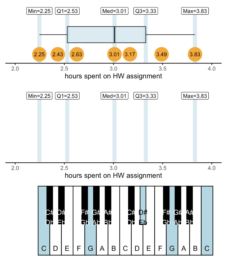
Sonifcations are generated via the custom function data_to_sonif(), which maps the largest value in the data set to a pre-specified low note, and the highest value to a pre-specified low note, then maps values in between maintaining the spacing between points rounded to the 12 tone equal tempered scale. For example, see how we sonify the five number summary to one octave:
Visualization of the pitch mapping sonification method.
Code
source("code/data_to_soniof_all.R")
Part 1: Just averages
The averages are sonified to a two octave range by mapping the lowest value to the low pitch of the range and the high note. As specified further below, the average will be played by a viola.
Code
## sonify first and last parts separately (so each part is scaled by its own max and min)sonif_all_mean =c(data_to_sonif_all(monthly_weather$mean[1:(change_date_part_2_index-1)], low =3, high =4),data_to_sonif_all(monthly_weather$mean[change_date_part_2_index:(change_date_part_3_index-1)], low =3, high =4),data_to_sonif_all(monthly_weather$mean[change_date_part_3_index:nrow(monthly_weather)], low =3, high =4) ) sonif_all_mean[change_date_part_2_index:(change_date_part_3_index-1)] <-NApattern =rep("eighth", times =length(sonif_all_mean))## lines for avg and max line_avg <-Line(pitches = sonif_all_mean, durations = pattern, name ="Monthly Average")
Part 2: Highs and Lows
The variability of the monthly maximum temperatures is slightly higher than that of the monthly minimum (Range of max: 57, Range of min:53 F; Standard deviation of max, min: 13.21 F, 8.54 F ). To represent this difference auditorially, we allow the maximum to span 3 octaves (C5 to C8) and the minumum to span 2 octaves (C3 to C5). Note that the minimum has the same octave span as the mean, which has a range of 40.5 F and a standard deviation of 9.21 F .
As defined below, the maximum is played by a celesta (a keyboard instrument) and the minimum is played by a bassoon.
Code
sonif_all_max =c(data_to_sonif_all(monthly_weather$max[1:(change_date_part_2_index-1)], low =5, high =7),data_to_sonif_all(monthly_weather$max[change_date_part_2_index:(change_date_part_3_index-1)], low =5, high =7),data_to_sonif_all(monthly_weather$max[change_date_part_3_index:nrow(monthly_weather)], low =5, high =7) ) sonif_all_max[1:change_date_part_2_index] <-NA## only average in part 1line_max <-Line(pitches = sonif_all_max, durations = pattern, name ="Monthly Max of Daily Maximum") ## create the musical linesonif_all_min =c(data_to_sonif_all(monthly_weather$min[1:(change_date_part_2_index-1)], low =3, high =4),data_to_sonif_all(monthly_weather$min[change_date_part_2_index:(change_date_part_3_index-1)], low =3, high =4),data_to_sonif_all(monthly_weather$min[change_date_part_3_index:nrow(monthly_weather)], low =3, high =4) ) sonif_all_min[1:change_date_part_2_index] <-NAline_min <-Line(pitches = sonif_all_min, durations = pattern, name ="Monthly Min of Daily Minimum")
Part 3: Exceedances
While it is an issue that temperatures on average are increasing, it is not audible on the scales played here since the change is very slow over time. However, the average is not the only statistic available to us, and in times of change we don’t necessarily want an estimate of just “typical” values.
One important tool for understanding how the extremes of a time series are changing over time are exceedance occurrances: tracking when a new high or a new low is hit.
If we just tracked new all time highs and lows, we would essentially only capture the worst winter/summer. Instead, we start the tracker at 1977 for reasons mentioned above,and track each season (Winter, Spring, Summer, Fall) so we see a sudden influx of “new” maximums and minumums as we begin the tracking, but then once we initialize we can then track when unusually high or low values occurr. I set the pitches at middle C for both to avoid the sonification becoming too busy.
As defined later, the exceedances occurrances are played with a viola to elevate the importance of exceedance occurrances as a statistic along with the average, which is also played by the viola.
Code
sonif_all_new_max =rep(NA, times =length(sonif_all_mean))sonif_all_new_max[monthly_weather$new_max] <-"C4"sonif_all_new_min =rep(NA, times =length(sonif_all_mean))sonif_all_new_min[monthly_weather$new_max] <-"C4"pattern_seas <-rep("quarter", times =length(sonif_all_max))line_max_new_seas <-Line(pitches = sonif_all_new_max, durations = pattern, name ="New Seasonal Maximum Reached")line_min_new_seas <-Line(pitches = sonif_all_new_max, durations = pattern, name ="New Seasonal Minimum Reached")
Create the music!
Here is where the instrumentation is actually added, and the music is outputted as an .mp3 file and/or score.
The choice of 12/8 time signature means that each measure is 1 year (12 months), with 4 beats felt per measure representing the four seasons, where each month is part of a seasonal triplet.
Contact Dr. Julia Schedler with questions or comments! Thanks for perceiving!
References
Flowers, John H., and Terry A. Hauer. 1993. “‘Sound’ Alternatives to Visual Graphics for Exploratory Data Analysis.”Behavior Research Methods, Instruments, & Computers 25 (2): 242–49. https://doi.org/10.3758/BF03204505.
Hermann, Thomas, Andrew Hunt, and John G. Neuhoff, eds. 2011. The Sonification Handbook. Berlin: Logos Verlag.
Peres, S Camille, and David M Lane. 2003. “SONIFICATIONOFSTATISTICALGRAPHS.” In Proceedings of the 2003 InternationalConference on AuditoryDisplay.
R Core Team. 2021. R: A Language and Environment for Statistical Computing. Vienna, Austria: R Foundation for Statistical Computing. https://www.R-project.org/.
Wickham, Hadley. 2016. Ggplot2: Elegant Graphics for Data Analysis. Springer-Verlag New York. https://ggplot2.tidyverse.org.
Footnotes
The gm package is absolutely delightful and I think anyone who can read music should look at the vignette and make R play their favorite lyric’s melody!↩︎